What’s the difference between the range and interquartile range?
While the range gives you the spread of the whole data set, the interquartile range gives you the spread of the middle half of a data set.
Frequently asked questions: Statistics
- What happens to the shape of Student’s t distribution as the degrees of freedom increase?
-
As the degrees of freedom increase, Student’s t distribution becomes less leptokurtic, meaning that the probability of extreme values decreases. The distribution becomes more and more similar to a standard normal distribution.
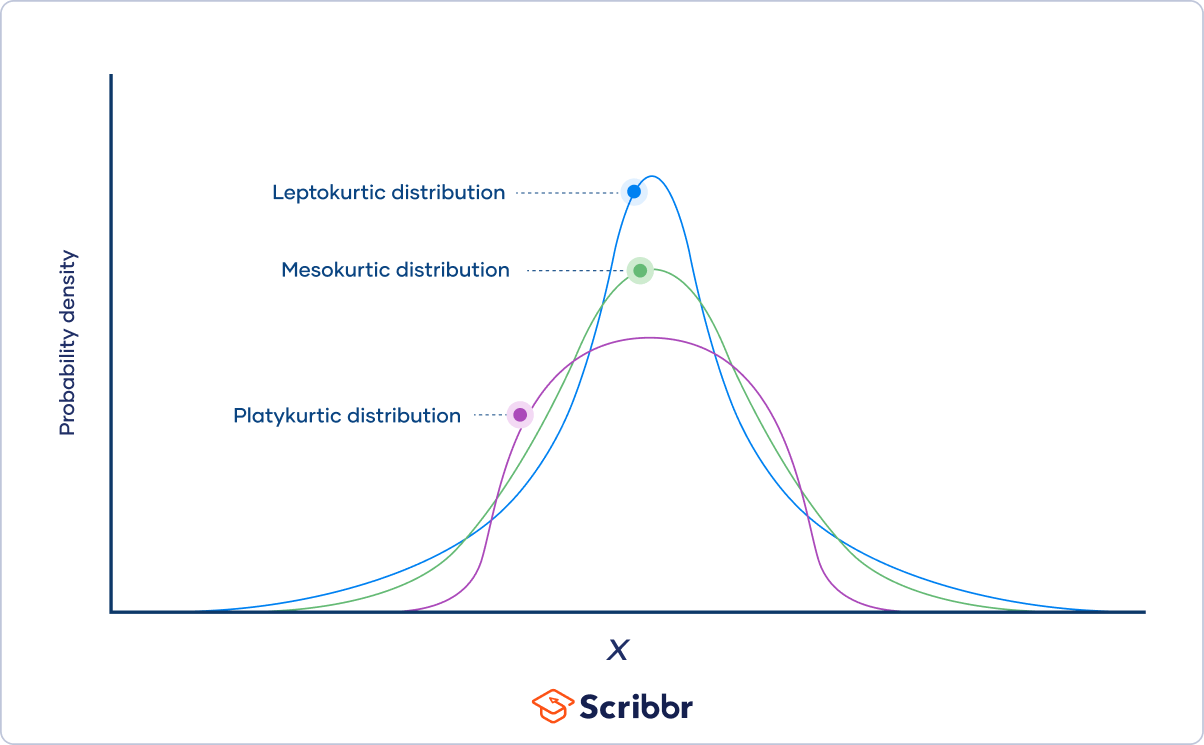
- What are the three categories of kurtosis?
-
The three categories of kurtosis are:
- Mesokurtosis: An excess kurtosis of 0. Normal distributions are mesokurtic.
- Platykurtosis: A negative excess kurtosis. Platykurtic distributions are thin-tailed, meaning that they have few outliers.
- Leptokurtosis: A positive excess kurtosis. Leptokurtic distributions are fat-tailed, meaning that they have many outliers.
- What are the two types of probability distributions?
-
Probability distributions belong to two broad categories: discrete probability distributions and continuous probability distributions. Within each category, there are many types of probability distributions.
- What’s the difference between relative frequency and probability?
-
Probability is the relative frequency over an infinite number of trials.
For example, the probability of a coin landing on heads is .5, meaning that if you flip the coin an infinite number of times, it will land on heads half the time.
Since doing something an infinite number of times is impossible, relative frequency is often used as an estimate of probability. If you flip a coin 1000 times and get 507 heads, the relative frequency, .507, is a good estimate of the probability.
- What types of data can be described by a frequency distribution?
-
Categorical variables can be described by a frequency distribution. Quantitative variables can also be described by a frequency distribution, but first they need to be grouped into interval classes.
- How can I tell if a frequency distribution appears to have a normal distribution?
-
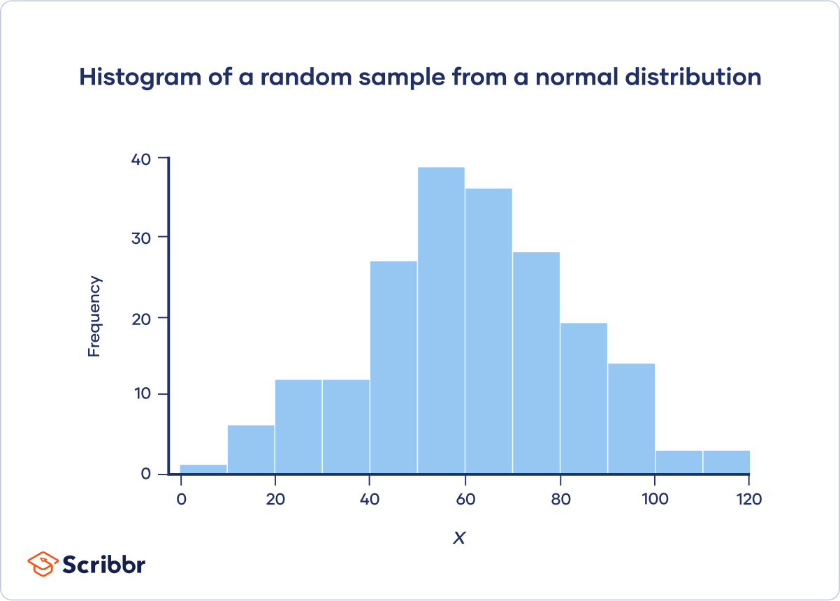
A histogram is an effective way to tell if a frequency distribution appears to have a normal distribution.
Plot a histogram and look at the shape of the bars. If the bars roughly follow a symmetrical bell or hill shape, like the example below, then the distribution is approximately normally distributed.

- How do I find a chi-square critical value in Excel?
-
You can use the CHISQ.INV.RT() function to find a chi-square critical value in Excel.
For example, to calculate the chi-square critical value for a test with df = 22 and α = .05, click any blank cell and type:
=CHISQ.INV.RT(0.05,22)
- How do I find a chi-square critical value in R?
-
You can use the qchisq() function to find a chi-square critical value in R.
For example, to calculate the chi-square critical value for a test with df = 22 and α = .05:
qchisq(p = .05, df = 22, lower.tail = FALSE)
- How do I perform a chi-square test of independence in R?
-
You can use the chisq.test() function to perform a chi-square test of independence in R. Give the contingency table as a matrix for the “x” argument. For example:
m = matrix(data = c(89, 84, 86, 9, 8, 24), nrow = 3, ncol = 2)
chisq.test(x = m)
- How do I perform a chi-square test of independence in Excel?
-
You can use the CHISQ.TEST() function to perform a chi-square test of independence in Excel. It takes two arguments, CHISQ.TEST(observed_range, expected_range), and returns the p value.
- How do I perform a chi-square goodness of fit test for a genetic cross?
-
Chi-square goodness of fit tests are often used in genetics. One common application is to check if two genes are linked (i.e., if the assortment is independent). When genes are linked, the allele inherited for one gene affects the allele inherited for another gene.
Suppose that you want to know if the genes for pea texture (R = round, r = wrinkled) and color (Y = yellow, y = green) are linked. You perform a dihybrid cross between two heterozygous (RY / ry) pea plants. The hypotheses you’re testing with your experiment are:
- Null hypothesis (H0): The population of offspring have an equal probability of inheriting all possible genotypic combinations.
- This would suggest that the genes are unlinked.
- Alternative hypothesis (Ha): The population of offspring do not have an equal probability of inheriting all possible genotypic combinations.
- This would suggest that the genes are linked.
You observe 100 peas:
- 78 round and yellow peas
- 6 round and green peas
- 4 wrinkled and yellow peas
- 12 wrinkled and green peas
Step 1: Calculate the expected frequencies
To calculate the expected values, you can make a Punnett square. If the two genes are unlinked, the probability of each genotypic combination is equal.
RY ry Ry rY RY RRYY RrYy RRYy RrYY ry RrYy rryy Rryy rrYy Ry RRYy Rryy RRyy RrYy rY RrYY rrYy RrYy rrYY The expected phenotypic ratios are therefore 9 round and yellow: 3 round and green: 3 wrinkled and yellow: 1 wrinkled and green.
From this, you can calculate the expected phenotypic frequencies for 100 peas:
Phenotype Observed Expected Round and yellow 78 100 * (9/16) = 56.25 Round and green 6 100 * (3/16) = 18.75 Wrinkled and yellow 4 100 * (3/16) = 18.75 Wrinkled and green 12 100 * (1/16) = 6.21 Step 2: Calculate chi-square
Phenotype Observed Expected O − E (O − E)2 (O − E)2 / E Round and yellow 78 56.25 21.75 473.06 8.41 Round and green 6 18.75 −12.75 162.56 8.67 Wrinkled and yellow 4 18.75 −14.75 217.56 11.6 Wrinkled and green 12 6.21 5.79 33.52 5.4 Χ2 = 8.41 + 8.67 + 11.6 + 5.4 = 34.08
Step 3: Find the critical chi-square value
Since there are four groups (round and yellow, round and green, wrinkled and yellow, wrinkled and green), there are three degrees of freedom.
For a test of significance at α = .05 and df = 3, the Χ2 critical value is 7.82.
Step 4: Compare the chi-square value to the critical value
Χ2 = 34.08
Critical value = 7.82
The Χ2 value is greater than the critical value.
Step 5: Decide whether the reject the null hypothesis
The Χ2 value is greater than the critical value, so we reject the null hypothesis that the population of offspring have an equal probability of inheriting all possible genotypic combinations. There is a significant difference between the observed and expected genotypic frequencies (p < .05).
The data supports the alternative hypothesis that the offspring do not have an equal probability of inheriting all possible genotypic combinations, which suggests that the genes are linked
- Null hypothesis (H0): The population of offspring have an equal probability of inheriting all possible genotypic combinations.
- How do I perform a chi-square goodness of fit test in R?
-
You can use the chisq.test() function to perform a chi-square goodness of fit test in R. Give the observed values in the “x” argument, give the expected values in the “p” argument, and set “rescale.p” to true. For example:
chisq.test(x = c(22,30,23), p = c(25,25,25), rescale.p = TRUE)
- How do I perform a chi-square goodness of fit test in Excel?
-
You can use the CHISQ.TEST() function to perform a chi-square goodness of fit test in Excel. It takes two arguments, CHISQ.TEST(observed_range, expected_range), and returns the p value.
- What is the difference between a chi-square test and a correlation?
-
Both correlations and chi-square tests can test for relationships between two variables. However, a correlation is used when you have two quantitative variables and a chi-square test of independence is used when you have two categorical variables.
- What is the difference between a chi-square test and a t test?
-
Both chi-square tests and t tests can test for differences between two groups. However, a t test is used when you have a dependent quantitative variable and an independent categorical variable (with two groups). A chi-square test of independence is used when you have two categorical variables.
- What are the two main types of chi-square tests?
-
The two main chi-square tests are the chi-square goodness of fit test and the chi-square test of independence.
- What properties does the chi-square distribution have?
-
A chi-square distribution is a continuous probability distribution. The shape of a chi-square distribution depends on its degrees of freedom, k. The mean of a chi-square distribution is equal to its degrees of freedom (k) and the variance is 2k. The range is 0 to ∞.
- What happens to the shape of the chi-square distribution as the degrees of freedom (k) increase?
-
As the degrees of freedom (k) increases, the chi-square distribution goes from a downward curve to a hump shape. As the degrees of freedom increases further, the hump goes from being strongly right-skewed to being approximately normal.
- How do I find the quartiles of a probability distribution?
-
To find the quartiles of a probability distribution, you can use the distribution’s quantile function.
- How do I find quartiles in R?
-
You can use the quantile() function to find quartiles in R. If your data is called “data”, then “quantile(data, prob=c(.25,.5,.75), type=1)” will return the three quartiles.
- How do I find quartiles in Excel?
-
You can use the QUARTILE() function to find quartiles in Excel. If your data is in column A, then click any blank cell and type “=QUARTILE(A:A,1)” for the first quartile, “=QUARTILE(A:A,2)” for the second quartile, and “=QUARTILE(A:A,3)” for the third quartile.
- How do I calculate the Pearson correlation coefficient in Excel?
-
You can use the PEARSON() function to calculate the Pearson correlation coefficient in Excel. If your variables are in columns A and B, then click any blank cell and type “PEARSON(A:A,B:B)”.
There is no function to directly test the significance of the correlation.
- How do I calculate the Pearson correlation coefficient in R?
-
You can use the cor() function to calculate the Pearson correlation coefficient in R. To test the significance of the correlation, you can use the cor.test() function.
- When should I use the Pearson correlation coefficient?
-
You should use the Pearson correlation coefficient when (1) the relationship is linear and (2) both variables are quantitative and (3) normally distributed and (4) have no outliers.
- What is the definition of the Pearson correlation coefficient?
-
The Pearson correlation coefficient (r) is the most common way of measuring a linear correlation. It is a number between –1 and 1 that measures the strength and direction of the relationship between two variables.
- What is the difference between a normal and a Poisson distribution?
-
This table summarizes the most important differences between normal distributions and Poisson distributions:
Characteristic Normal Poisson Continuous or discrete Continuous Discrete Parameter Mean (µ) and standard deviation (σ) Lambda (λ) Shape Bell-shaped Depends on λ Symmetry Symmetrical Asymmetrical (right-skewed). As λ increases, the asymmetry decreases. Range −∞ to ∞ 0 to ∞ When the mean of a Poisson distribution is large (>10), it can be approximated by a normal distribution.
- What does lambda (λ) mean in the Poisson distribution formula?
-
In the Poisson distribution formula, lambda (λ) is the mean number of events within a given interval of time or space. For example, λ = 0.748 floods per year.
- What does “e” mean in the Poisson distribution formula?
-
The e in the Poisson distribution formula stands for the number 2.718. This number is called Euler’s constant. You can simply substitute e with 2.718 when you’re calculating a Poisson probability. Euler’s constant is a very useful number and is especially important in calculus.
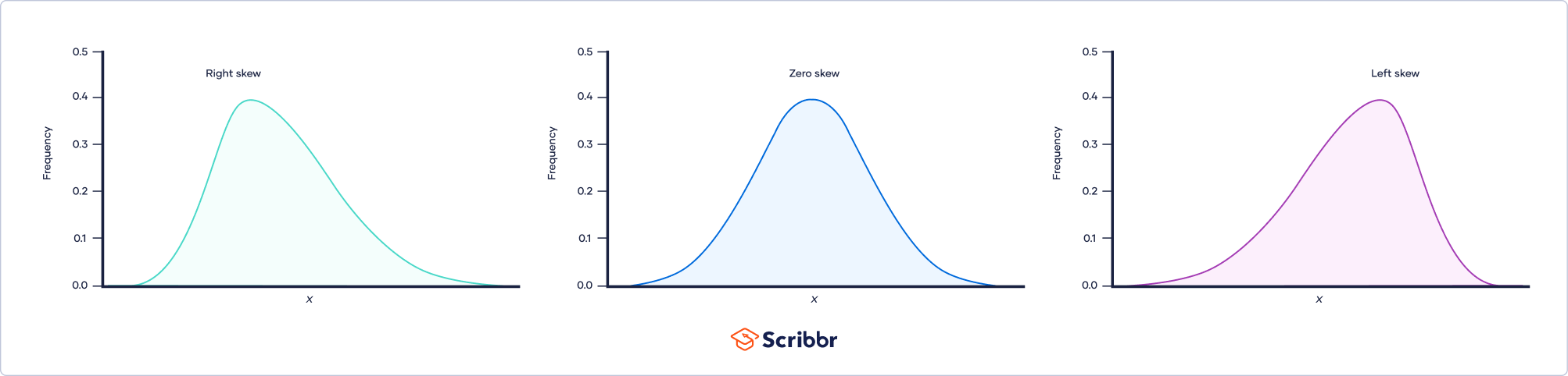
- What are the three types of skewness?
-
The three types of skewness are:
- Right skew (also called positive skew). A right-skewed distribution is longer on the right side of its peak than on its left.
- Left skew (also called negative skew). A left-skewed distribution is longer on the left side of its peak than on its right.
- Zero skew. It is symmetrical and its left and right sides are mirror images.

- What is the difference between skewness and kurtosis?
-
Skewness and kurtosis are both important measures of a distribution’s shape.
- Skewness measures the asymmetry of a distribution.
- Kurtosis measures the heaviness of a distribution’s tails relative to a normal distribution.

- What’s the difference between a research hypothesis and a statistical hypothesis?
-
A research hypothesis is your proposed answer to your research question. The research hypothesis usually includes an explanation (“x affects y because …”).
A statistical hypothesis, on the other hand, is a mathematical statement about a population parameter. Statistical hypotheses always come in pairs: the null and alternative hypotheses. In a well-designed study, the statistical hypotheses correspond logically to the research hypothesis.
- What symbols are used to represent alternative hypotheses?
-
The alternative hypothesis is often abbreviated as Ha or H1. When the alternative hypothesis is written using mathematical symbols, it always includes an inequality symbol (usually ≠, but sometimes < or >).
- What symbols are used to represent null hypotheses?
-
The null hypothesis is often abbreviated as H0. When the null hypothesis is written using mathematical symbols, it always includes an equality symbol (usually =, but sometimes ≥ or ≤).
- Why is the t distribution also called Student’s t distribution?
-
The t distribution was first described by statistician William Sealy Gosset under the pseudonym “Student.”
- How do I calculate a confidence interval of a mean using the critical value of t?
-
To calculate a confidence interval of a mean using the critical value of t, follow these four steps:
- Choose the significance level based on your desired confidence level. The most common confidence level is 95%, which corresponds to α = .05 in the two-tailed t table.
- Find the critical value of t in the two-tailed t table.
- Multiply the critical value of t by s/√n.
- Add this value to the mean to calculate the upper limit of the confidence interval, and subtract this value from the mean to calculate the lower limit.
- How do I test a hypothesis using the critical value of t?
-
To test a hypothesis using the critical value of t, follow these four steps:
- Calculate the t value for your sample.
- Find the critical value of t in the t table.
- Determine if the (absolute) t value is greater than the critical value of t.
- Reject the null hypothesis if the sample’s t value is greater than the critical value of t. Otherwise, don’t reject the null hypothesis.
- How do I find the critical value of t in Excel?
-
You can use the T.INV() function to find the critical value of t for one-tailed tests in Excel, and you can use the T.INV.2T() function for two-tailed tests.
Example: Calculating the critical value of t in Excel To calculate the critical value of t for a two-tailed test with df = 29 and α = .05, click any blank cell and type:=T.INV.2T(0.05,29)
- How do I find the critical value of t in R?
-
You can use the qt() function to find the critical value of t in R. The function gives the critical value of t for the one-tailed test. If you want the critical value of t for a two-tailed test, divide the significance level by two.
Example: Calculating the critical value of t in R To calculate the critical value of t for a two-tailed test with df = 29 and α = .05:qt(p = .025, df = 29)
- How do I calculate the coefficient of determination (R²) in Excel?
-
You can use the RSQ() function to calculate R² in Excel. If your dependent variable is in column A and your independent variable is in column B, then click any blank cell and type “RSQ(A:A,B:B)”.
- How do I calculate the coefficient of determination (R²) in R?
-
You can use the summary() function to view the R² of a linear model in R. You will see the “R-squared” near the bottom of the output.
- What is the formula for the coefficient of determination (R²)?
-
There are two formulas you can use to calculate the coefficient of determination (R²) of a simple linear regression.
Formula 1:

Formula 2:

- What is the definition of the coefficient of determination (R²)?
-
The coefficient of determination (R²) is a number between 0 and 1 that measures how well a statistical model predicts an outcome. You can interpret the R² as the proportion of variation in the dependent variable that is predicted by the statistical model.
- What are the types of missing data?
-
There are three main types of missing data.
Missing completely at random (MCAR) data are randomly distributed across the variable and unrelated to other variables.
Missing at random (MAR) data are not randomly distributed but they are accounted for by other observed variables.
Missing not at random (MNAR) data systematically differ from the observed values.
- How do I deal with missing data?
-
To tidy up your missing data, your options usually include accepting, removing, or recreating the missing data.
- Acceptance: You leave your data as is
- Listwise or pairwise deletion: You delete all cases (participants) with missing data from analyses
- Imputation: You use other data to fill in the missing data
- Why are missing data important?
-
Missing data are important because, depending on the type, they can sometimes bias your results. This means your results may not be generalizable outside of your study because your data come from an unrepresentative sample.
- What are missing data?
-
Missing data, or missing values, occur when you don’t have data stored for certain variables or participants.
In any dataset, there’s usually some missing data. In quantitative research, missing values appear as blank cells in your spreadsheet.
- How do I calculate the geometric mean?
-
There are two steps to calculating the geometric mean:
- Multiply all values together to get their product.
- Find the nth root of the product (n is the number of values).
Before calculating the geometric mean, note that:
- The geometric mean can only be found for positive values.
- If any value in the data set is zero, the geometric mean is zero.
- What’s the difference between the arithmetic and geometric means?
-
The arithmetic mean is the most commonly used type of mean and is often referred to simply as “the mean.” While the arithmetic mean is based on adding and dividing values, the geometric mean multiplies and finds the root of values.
Even though the geometric mean is a less common measure of central tendency, it’s more accurate than the arithmetic mean for percentage change and positively skewed data. The geometric mean is often reported for financial indices and population growth rates.
- What is the geometric mean?
-
The geometric mean is an average that multiplies all values and finds a root of the number. For a dataset with n numbers, you find the nth root of their product.
- What are outliers?
-
Outliers are extreme values that differ from most values in the dataset. You find outliers at the extreme ends of your dataset.
- When should I remove an outlier from my dataset?
-
It’s best to remove outliers only when you have a sound reason for doing so.
Some outliers represent natural variations in the population, and they should be left as is in your dataset. These are called true outliers.
Other outliers are problematic and should be removed because they represent measurement errors, data entry or processing errors, or poor sampling.
- How do I find outliers in my data?
-
You can choose from four main ways to detect outliers:
- Sorting your values from low to high and checking minimum and maximum values
- Visualizing your data with a box plot and looking for outliers
- Using the interquartile range to create fences for your data
- Using statistical procedures to identify extreme values
- Why do outliers matter?
-
Outliers can have a big impact on your statistical analyses and skew the results of any hypothesis test if they are inaccurate.
These extreme values can impact your statistical power as well, making it hard to detect a true effect if there is one.
- Is the correlation coefficient the same as the slope of the line?
-
No, the steepness or slope of the line isn’t related to the correlation coefficient value. The correlation coefficient only tells you how closely your data fit on a line, so two datasets with the same correlation coefficient can have very different slopes.
To find the slope of the line, you’ll need to perform a regression analysis.
- What do the sign and value of the correlation coefficient tell you?
-
Correlation coefficients always range between -1 and 1.
The sign of the coefficient tells you the direction of the relationship: a positive value means the variables change together in the same direction, while a negative value means they change together in opposite directions.
The absolute value of a number is equal to the number without its sign. The absolute value of a correlation coefficient tells you the magnitude of the correlation: the greater the absolute value, the stronger the correlation.
- What are the assumptions of the Pearson correlation coefficient?
-
These are the assumptions your data must meet if you want to use Pearson’s r:
- Both variables are on an interval or ratio level of measurement
- Data from both variables follow normal distributions
- Your data have no outliers
- Your data is from a random or representative sample
- You expect a linear relationship between the two variables
- What is a correlation coefficient?
-
A correlation coefficient is a single number that describes the strength and direction of the relationship between your variables.
Different types of correlation coefficients might be appropriate for your data based on their levels of measurement and distributions. The Pearson product-moment correlation coefficient (Pearson’s r) is commonly used to assess a linear relationship between two quantitative variables.
- How do you increase statistical power?
-
There are various ways to improve power:
- Increase the potential effect size by manipulating your independent variable more strongly,
- Increase sample size,
- Increase the significance level (alpha),
- Reduce measurement error by increasing the precision and accuracy of your measurement devices and procedures,
- Use a one-tailed test instead of a two-tailed test for t tests and z tests.
- What is a power analysis?
-
A power analysis is a calculation that helps you determine a minimum sample size for your study. It’s made up of four main components. If you know or have estimates for any three of these, you can calculate the fourth component.
- Statistical power: the likelihood that a test will detect an effect of a certain size if there is one, usually set at 80% or higher.
- Sample size: the minimum number of observations needed to observe an effect of a certain size with a given power level.
- Significance level (alpha): the maximum risk of rejecting a true null hypothesis that you are willing to take, usually set at 5%.
- Expected effect size: a standardized way of expressing the magnitude of the expected result of your study, usually based on similar studies or a pilot study.
- What are null and alternative hypotheses?
-
Null and alternative hypotheses are used in statistical hypothesis testing. The null hypothesis of a test always predicts no effect or no relationship between variables, while the alternative hypothesis states your research prediction of an effect or relationship.
- What is statistical analysis?
-
Statistical analysis is the main method for analyzing quantitative research data. It uses probabilities and models to test predictions about a population from sample data.
- How do you reduce the risk of making a Type II error?
-
The risk of making a Type II error is inversely related to the statistical power of a test. Power is the extent to which a test can correctly detect a real effect when there is one.
To (indirectly) reduce the risk of a Type II error, you can increase the sample size or the significance level to increase statistical power.
- How do you reduce the risk of making a Type I error?
-
The risk of making a Type I error is the significance level (or alpha) that you choose. That’s a value that you set at the beginning of your study to assess the statistical probability of obtaining your results (p value).
The significance level is usually set at 0.05 or 5%. This means that your results only have a 5% chance of occurring, or less, if the null hypothesis is actually true.
To reduce the Type I error probability, you can set a lower significance level.
- What are Type I and Type II errors?
-
In statistics, a Type I error means rejecting the null hypothesis when it’s actually true, while a Type II error means failing to reject the null hypothesis when it’s actually false.
- What is statistical power?
-
In statistics, power refers to the likelihood of a hypothesis test detecting a true effect if there is one. A statistically powerful test is more likely to reject a false negative (a Type II error).
If you don’t ensure enough power in your study, you may not be able to detect a statistically significant result even when it has practical significance. Your study might not have the ability to answer your research question.
- What’s the difference between statistical and practical significance?
-
While statistical significance shows that an effect exists in a study, practical significance shows that the effect is large enough to be meaningful in the real world.
Statistical significance is denoted by p-values whereas practical significance is represented by effect sizes.
- How do I calculate effect size?
-
There are dozens of measures of effect sizes. The most common effect sizes are Cohen’s d and Pearson’s r. Cohen’s d measures the size of the difference between two groups while Pearson’s r measures the strength of the relationship between two variables.
- What is effect size?
-
Effect size tells you how meaningful the relationship between variables or the difference between groups is.
A large effect size means that a research finding has practical significance, while a small effect size indicates limited practical applications.
- What’s the difference between a point estimate and an interval estimate?
-
Using descriptive and inferential statistics, you can make two types of estimates about the population: point estimates and interval estimates.
- A point estimate is a single value estimate of a parameter. For instance, a sample mean is a point estimate of a population mean.
- An interval estimate gives you a range of values where the parameter is expected to lie. A confidence interval is the most common type of interval estimate.
Both types of estimates are important for gathering a clear idea of where a parameter is likely to lie.
- What’s the difference between standard error and standard deviation?
-
Standard error and standard deviation are both measures of variability. The standard deviation reflects variability within a sample, while the standard error estimates the variability across samples of a population.
- What is standard error?
-
The standard error of the mean, or simply standard error, indicates how different the population mean is likely to be from a sample mean. It tells you how much the sample mean would vary if you were to repeat a study using new samples from within a single population.
- How do you know whether a number is a parameter or a statistic?
-
To figure out whether a given number is a parameter or a statistic, ask yourself the following:
- Does the number describe a whole, complete population where every member can be reached for data collection?
- Is it possible to collect data for this number from every member of the population in a reasonable time frame?
If the answer is yes to both questions, the number is likely to be a parameter. For small populations, data can be collected from the whole population and summarized in parameters.
If the answer is no to either of the questions, then the number is more likely to be a statistic.
- What are the different types of means?
-
The arithmetic mean is the most commonly used mean. It’s often simply called the mean or the average. But there are some other types of means you can calculate depending on your research purposes:
- Weighted mean: some values contribute more to the mean than others.
- Geometric mean: values are multiplied rather than summed up.
- Harmonic mean: reciprocals of values are used instead of the values themselves.
- How do I find the mean?
-
You can find the mean, or average, of a data set in two simple steps:
- Find the sum of the values by adding them all up.
- Divide the sum by the number of values in the data set.
This method is the same whether you are dealing with sample or population data or positive or negative numbers.
- When should I use the median?
-
The median is the most informative measure of central tendency for skewed distributions or distributions with outliers. For example, the median is often used as a measure of central tendency for income distributions, which are generally highly skewed.
Because the median only uses one or two values, it’s unaffected by extreme outliers or non-symmetric distributions of scores. In contrast, the mean and mode can vary in skewed distributions.
- How do I find the median?
-
To find the median, first order your data. Then calculate the middle position based on n, the number of values in your data set.
- If n is an odd number, the median lies at the position
 .
. - If n is an even number, the median is the mean of the values at positions
 and
and  .
.
- If n is an odd number, the median lies at the position
- Can there be more than one mode?
-
A data set can often have no mode, one mode or more than one mode – it all depends on how many different values repeat most frequently.
Your data can be:
- without any mode
- unimodal, with one mode,
- bimodal, with two modes,
- trimodal, with three modes, or
- multimodal, with four or more modes.
- How do I find the mode?
-
To find the mode:
- If your data is numerical or quantitative, order the values from low to high.
- If it is categorical, sort the values by group, in any order.
Then you simply need to identify the most frequently occurring value.
- When should I use the interquartile range?
-
The interquartile range is the best measure of variability for skewed distributions or data sets with outliers. Because it’s based on values that come from the middle half of the distribution, it’s unlikely to be influenced by outliers.
- What are the two main methods for calculating interquartile range?
-
The two most common methods for calculating interquartile range are the exclusive and inclusive methods.
The exclusive method excludes the median when identifying Q1 and Q3, while the inclusive method includes the median as a value in the data set in identifying the quartiles.
For each of these methods, you’ll need different procedures for finding the median, Q1 and Q3 depending on whether your sample size is even- or odd-numbered. The exclusive method works best for even-numbered sample sizes, while the inclusive method is often used with odd-numbered sample sizes.
- What is homoscedasticity?
-
Homoscedasticity, or homogeneity of variances, is an assumption of equal or similar variances in different groups being compared.
This is an important assumption of parametric statistical tests because they are sensitive to any dissimilarities. Uneven variances in samples result in biased and skewed test results.
- What is variance used for in statistics?
-
Statistical tests such as variance tests or the analysis of variance (ANOVA) use sample variance to assess group differences of populations. They use the variances of the samples to assess whether the populations they come from significantly differ from each other.
- What’s the difference between standard deviation and variance?
-
Variance is the average squared deviations from the mean, while standard deviation is the square root of this number. Both measures reflect variability in a distribution, but their units differ:
- Standard deviation is expressed in the same units as the original values (e.g., minutes or meters).
- Variance is expressed in much larger units (e.g., meters squared).
Although the units of variance are harder to intuitively understand, variance is important in statistical tests.
- What is the empirical rule?
-
The empirical rule, or the 68-95-99.7 rule, tells you where most of the values lie in a normal distribution:
- Around 68% of values are within 1 standard deviation of the mean.
- Around 95% of values are within 2 standard deviations of the mean.
- Around 99.7% of values are within 3 standard deviations of the mean.
The empirical rule is a quick way to get an overview of your data and check for any outliers or extreme values that don’t follow this pattern.
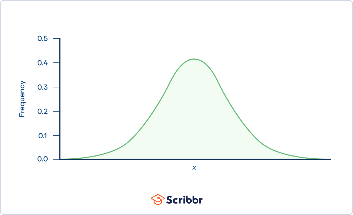
- What is a normal distribution?
-
In a normal distribution, data are symmetrically distributed with no skew. Most values cluster around a central region, with values tapering off as they go further away from the center.
The measures of central tendency (mean, mode, and median) are exactly the same in a normal distribution.
- What does standard deviation tell you?
-
The standard deviation is the average amount of variability in your data set. It tells you, on average, how far each score lies from the mean.
In normal distributions, a high standard deviation means that values are generally far from the mean, while a low standard deviation indicates that values are clustered close to the mean.
- Can the range be a negative number?
-
No. Because the range formula subtracts the lowest number from the highest number, the range is always zero or a positive number.
- What is the range in statistics?
-
In statistics, the range is the spread of your data from the lowest to the highest value in the distribution. It is the simplest measure of variability.
- What’s the difference between central tendency and variability?
-
While central tendency tells you where most of your data points lie, variability summarizes how far apart your points from each other.
Data sets can have the same central tendency but different levels of variability or vice versa. Together, they give you a complete picture of your data.
- What are the 4 main measures of variability?
-
Variability is most commonly measured with the following descriptive statistics:
- Range: the difference between the highest and lowest values
- Interquartile range: the range of the middle half of a distribution
- Standard deviation: average distance from the mean
- Variance: average of squared distances from the mean
- What is variability?
-
Variability tells you how far apart points lie from each other and from the center of a distribution or a data set.
Variability is also referred to as spread, scatter or dispersion.
- What is the difference between interval and ratio data?
-
While interval and ratio data can both be categorized, ranked, and have equal spacing between adjacent values, only ratio scales have a true zero.
For example, temperature in Celsius or Fahrenheit is at an interval scale because zero is not the lowest possible temperature. In the Kelvin scale, a ratio scale, zero represents a total lack of thermal energy.
- What is a critical value?
-
A critical value is the value of the test statistic which defines the upper and lower bounds of a confidence interval, or which defines the threshold of statistical significance in a statistical test. It describes how far from the mean of the distribution you have to go to cover a certain amount of the total variation in the data (i.e. 90%, 95%, 99%).
If you are constructing a 95% confidence interval and are using a threshold of statistical significance of p = 0.05, then your critical value will be identical in both cases.
- What is the difference between the t-distribution and the standard normal distribution?
-
The t-distribution gives more probability to observations in the tails of the distribution than the standard normal distribution (a.k.a. the z-distribution).
In this way, the t-distribution is more conservative than the standard normal distribution: to reach the same level of confidence or statistical significance, you will need to include a wider range of the data.
- What is a t-score?
-
A t-score (a.k.a. a t-value) is equivalent to the number of standard deviations away from the mean of the t-distribution.
The t-score is the test statistic used in t-tests and regression tests. It can also be used to describe how far from the mean an observation is when the data follow a t-distribution.
- What is a t-distribution?
-
The t-distribution is a way of describing a set of observations where most observations fall close to the mean, and the rest of the observations make up the tails on either side. It is a type of normal distribution used for smaller sample sizes, where the variance in the data is unknown.
The t-distribution forms a bell curve when plotted on a graph. It can be described mathematically using the mean and the standard deviation.
- Are ordinal variables categorical or quantitative?
-
In statistics, ordinal and nominal variables are both considered categorical variables.
Even though ordinal data can sometimes be numerical, not all mathematical operations can be performed on them.
- What is ordinal data?
-
Ordinal data has two characteristics:
- The data can be classified into different categories within a variable.
- The categories have a natural ranked order.
However, unlike with interval data, the distances between the categories are uneven or unknown.
- What’s the difference between nominal and ordinal data?
-
Nominal and ordinal are two of the four levels of measurement. Nominal level data can only be classified, while ordinal level data can be classified and ordered.
- What is nominal data?
-
Nominal data is data that can be labelled or classified into mutually exclusive categories within a variable. These categories cannot be ordered in a meaningful way.
For example, for the nominal variable of preferred mode of transportation, you may have the categories of car, bus, train, tram or bicycle.
- What does it mean if my confidence interval includes zero?
-
If your confidence interval for a difference between groups includes zero, that means that if you run your experiment again you have a good chance of finding no difference between groups.
If your confidence interval for a correlation or regression includes zero, that means that if you run your experiment again there is a good chance of finding no correlation in your data.
In both of these cases, you will also find a high p-value when you run your statistical test, meaning that your results could have occurred under the null hypothesis of no relationship between variables or no difference between groups.
- How do I calculate a confidence interval if my data are not normally distributed?
-
If you want to calculate a confidence interval around the mean of data that is not normally distributed, you have two choices:
- Find a distribution that matches the shape of your data and use that distribution to calculate the confidence interval.
- Perform a transformation on your data to make it fit a normal distribution, and then find the confidence interval for the transformed data.
- What is a standard normal distribution?
-
The standard normal distribution, also called the z-distribution, is a special normal distribution where the mean is 0 and the standard deviation is 1.
Any normal distribution can be converted into the standard normal distribution by turning the individual values into z-scores. In a z-distribution, z-scores tell you how many standard deviations away from the mean each value lies.
- What are z-scores and t-scores?
-
The z-score and t-score (aka z-value and t-value) show how many standard deviations away from the mean of the distribution you are, assuming your data follow a z-distribution or a t-distribution.
These scores are used in statistical tests to show how far from the mean of the predicted distribution your statistical estimate is. If your test produces a z-score of 2.5, this means that your estimate is 2.5 standard deviations from the predicted mean.
The predicted mean and distribution of your estimate are generated by the null hypothesis of the statistical test you are using. The more standard deviations away from the predicted mean your estimate is, the less likely it is that the estimate could have occurred under the null hypothesis.
- How do you calculate a confidence interval?
-
To calculate the confidence interval, you need to know:
- The point estimate you are constructing the confidence interval for
- The critical values for the test statistic
- The standard deviation of the sample
- The sample size
Then you can plug these components into the confidence interval formula that corresponds to your data. The formula depends on the type of estimate (e.g. a mean or a proportion) and on the distribution of your data.
- What is the difference between a confidence interval and a confidence level?
-
The confidence level is the percentage of times you expect to get close to the same estimate if you run your experiment again or resample the population in the same way.
The confidence interval consists of the upper and lower bounds of the estimate you expect to find at a given level of confidence.
For example, if you are estimating a 95% confidence interval around the mean proportion of female babies born every year based on a random sample of babies, you might find an upper bound of 0.56 and a lower bound of 0.48. These are the upper and lower bounds of the confidence interval. The confidence level is 95%.
- What’s the best measure of central tendency to use?
-
The mean is the most frequently used measure of central tendency because it uses all values in the data set to give you an average.
For data from skewed distributions, the median is better than the mean because it isn’t influenced by extremely large values.
The mode is the only measure you can use for nominal or categorical data that can’t be ordered.
- Which measures of central tendency can I use?
-
The measures of central tendency you can use depends on the level of measurement of your data.
- For a nominal level, you can only use the mode to find the most frequent value.
- For an ordinal level or ranked data, you can also use the median to find the value in the middle of your data set.
- For interval or ratio levels, in addition to the mode and median, you can use the mean to find the average value.
- What are measures of central tendency?
-
Measures of central tendency help you find the middle, or the average, of a data set.
The 3 most common measures of central tendency are the mean, median and mode.
- How do I decide which level of measurement to use?
-
Some variables have fixed levels. For example, gender and ethnicity are always nominal level data because they cannot be ranked.
However, for other variables, you can choose the level of measurement. For example, income is a variable that can be recorded on an ordinal or a ratio scale:
- At an ordinal level, you could create 5 income groupings and code the incomes that fall within them from 1–5.
- At a ratio level, you would record exact numbers for income.
If you have a choice, the ratio level is always preferable because you can analyze data in more ways. The higher the level of measurement, the more precise your data is.
- Why do levels of measurement matter?
-
The level at which you measure a variable determines how you can analyze your data.
Depending on the level of measurement, you can perform different descriptive statistics to get an overall summary of your data and inferential statistics to see if your results support or refute your hypothesis.
- What are the four levels of measurement?
-
Levels of measurement tell you how precisely variables are recorded. There are 4 levels of measurement, which can be ranked from low to high:
- Does a p-value tell you whether your alternative hypothesis is true?
-
No. The p-value only tells you how likely the data you have observed is to have occurred under the null hypothesis.
If the p-value is below your threshold of significance (typically p < 0.05), then you can reject the null hypothesis, but this does not necessarily mean that your alternative hypothesis is true.
- Which alpha value should I use?
-
The alpha value, or the threshold for statistical significance, is arbitrary – which value you use depends on your field of study.
In most cases, researchers use an alpha of 0.05, which means that there is a less than 5% chance that the data being tested could have occurred under the null hypothesis.
- How do you calculate a p-value?
-
P-values are usually automatically calculated by the program you use to perform your statistical test. They can also be estimated using p-value tables for the relevant test statistic.
P-values are calculated from the null distribution of the test statistic. They tell you how often a test statistic is expected to occur under the null hypothesis of the statistical test, based on where it falls in the null distribution.
If the test statistic is far from the mean of the null distribution, then the p-value will be small, showing that the test statistic is not likely to have occurred under the null hypothesis.
- What is a p-value?
-
A p-value, or probability value, is a number describing how likely it is that your data would have occurred under the null hypothesis of your statistical test.
- How do I know which test statistic to use?
-
The test statistic you use will be determined by the statistical test.
You can choose the right statistical test by looking at what type of data you have collected and what type of relationship you want to test.
- What factors affect the test statistic?
-
The test statistic will change based on the number of observations in your data, how variable your observations are, and how strong the underlying patterns in the data are.
For example, if one data set has higher variability while another has lower variability, the first data set will produce a test statistic closer to the null hypothesis, even if the true correlation between two variables is the same in either data set.
- How do you calculate a test statistic?
-
The formula for the test statistic depends on the statistical test being used.
Generally, the test statistic is calculated as the pattern in your data (i.e. the correlation between variables or difference between groups) divided by the variance in the data (i.e. the standard deviation).
- What’s the difference between univariate, bivariate and multivariate descriptive statistics?
-
- Univariate statistics summarize only one variable at a time.
- Bivariate statistics compare two variables.
- Multivariate statistics compare more than two variables.
- What are the 3 main types of descriptive statistics?
-
The 3 main types of descriptive statistics concern the frequency distribution, central tendency, and variability of a dataset.
- Distribution refers to the frequencies of different responses.
- Measures of central tendency give you the average for each response.
- Measures of variability show you the spread or dispersion of your dataset.
- What’s the difference between descriptive and inferential statistics?
-
Descriptive statistics summarize the characteristics of a data set. Inferential statistics allow you to test a hypothesis or assess whether your data is generalizable to the broader population.
- What is meant by model selection?
-
In statistics, model selection is a process researchers use to compare the relative value of different statistical models and determine which one is the best fit for the observed data.
The Akaike information criterion is one of the most common methods of model selection. AIC weights the ability of the model to predict the observed data against the number of parameters the model requires to reach that level of precision.
AIC model selection can help researchers find a model that explains the observed variation in their data while avoiding overfitting.
- What is a model?
-
In statistics, a model is the collection of one or more independent variables and their predicted interactions that researchers use to try to explain variation in their dependent variable.
You can test a model using a statistical test. To compare how well different models fit your data, you can use Akaike’s information criterion for model selection.
- How is AIC calculated?
-
The Akaike information criterion is calculated from the maximum log-likelihood of the model and the number of parameters (K) used to reach that likelihood. The AIC function is 2K – 2(log-likelihood).
Lower AIC values indicate a better-fit model, and a model with a delta-AIC (the difference between the two AIC values being compared) of more than -2 is considered significantly better than the model it is being compared to.
- What is the Akaike information criterion?
-
The Akaike information criterion is a mathematical test used to evaluate how well a model fits the data it is meant to describe. It penalizes models which use more independent variables (parameters) as a way to avoid over-fitting.
AIC is most often used to compare the relative goodness-of-fit among different models under consideration and to then choose the model that best fits the data.
- What is a factorial ANOVA?
-
A factorial ANOVA is any ANOVA that uses more than one categorical independent variable. A two-way ANOVA is a type of factorial ANOVA.
Some examples of factorial ANOVAs include:
- Testing the combined effects of vaccination (vaccinated or not vaccinated) and health status (healthy or pre-existing condition) on the rate of flu infection in a population.
- Testing the effects of marital status (married, single, divorced, widowed), job status (employed, self-employed, unemployed, retired), and family history (no family history, some family history) on the incidence of depression in a population.
- Testing the effects of feed type (type A, B, or C) and barn crowding (not crowded, somewhat crowded, very crowded) on the final weight of chickens in a commercial farming operation.
- How is statistical significance calculated in an ANOVA?
-
In ANOVA, the null hypothesis is that there is no difference among group means. If any group differs significantly from the overall group mean, then the ANOVA will report a statistically significant result.
Significant differences among group means are calculated using the F statistic, which is the ratio of the mean sum of squares (the variance explained by the independent variable) to the mean square error (the variance left over).
If the F statistic is higher than the critical value (the value of F that corresponds with your alpha value, usually 0.05), then the difference among groups is deemed statistically significant.
- What is the difference between a one-way and a two-way ANOVA?
-
The only difference between one-way and two-way ANOVA is the number of independent variables. A one-way ANOVA has one independent variable, while a two-way ANOVA has two.
- One-way ANOVA: Testing the relationship between shoe brand (Nike, Adidas, Saucony, Hoka) and race finish times in a marathon.
- Two-way ANOVA: Testing the relationship between shoe brand (Nike, Adidas, Saucony, Hoka), runner age group (junior, senior, master’s), and race finishing times in a marathon.
All ANOVAs are designed to test for differences among three or more groups. If you are only testing for a difference between two groups, use a t-test instead.
- What is multiple linear regression?
-
Multiple linear regression is a regression model that estimates the relationship between a quantitative dependent variable and two or more independent variables using a straight line.
- How is the error calculated in a linear regression model?
-
Linear regression most often uses mean-square error (MSE) to calculate the error of the model. MSE is calculated by:
- measuring the distance of the observed y-values from the predicted y-values at each value of x;
- squaring each of these distances;
- calculating the mean of each of the squared distances.
Linear regression fits a line to the data by finding the regression coefficient that results in the smallest MSE.
- What is simple linear regression?
-
Simple linear regression is a regression model that estimates the relationship between one independent variable and one dependent variable using a straight line. Both variables should be quantitative.
For example, the relationship between temperature and the expansion of mercury in a thermometer can be modeled using a straight line: as temperature increases, the mercury expands. This linear relationship is so certain that we can use mercury thermometers to measure temperature.
- What is a regression model?
-
A regression model is a statistical model that estimates the relationship between one dependent variable and one or more independent variables using a line (or a plane in the case of two or more independent variables).
A regression model can be used when the dependent variable is quantitative, except in the case of logistic regression, where the dependent variable is binary.
- Can I use a t-test to measure the difference among several groups?
-
A t-test should not be used to measure differences among more than two groups, because the error structure for a t-test will underestimate the actual error when many groups are being compared.
If you want to compare the means of several groups at once, it’s best to use another statistical test such as ANOVA or a post-hoc test.
- What is the difference between a one-sample t-test and a paired t-test?
-
A one-sample t-test is used to compare a single population to a standard value (for example, to determine whether the average lifespan of a specific town is different from the country average).
A paired t-test is used to compare a single population before and after some experimental intervention or at two different points in time (for example, measuring student performance on a test before and after being taught the material).
- What does a t-test measure?
-
A t-test measures the difference in group means divided by the pooled standard error of the two group means.
In this way, it calculates a number (the t-value) illustrating the magnitude of the difference between the two group means being compared, and estimates the likelihood that this difference exists purely by chance (p-value).
- Which t-test should I use?
-
Your choice of t-test depends on whether you are studying one group or two groups, and whether you care about the direction of the difference in group means.
If you are studying one group, use a paired t-test to compare the group mean over time or after an intervention, or use a one-sample t-test to compare the group mean to a standard value. If you are studying two groups, use a two-sample t-test.
If you want to know only whether a difference exists, use a two-tailed test. If you want to know if one group mean is greater or less than the other, use a left-tailed or right-tailed one-tailed test.
- What is a t-test?
-
A t-test is a statistical test that compares the means of two samples. It is used in hypothesis testing, with a null hypothesis that the difference in group means is zero and an alternate hypothesis that the difference in group means is different from zero.
- What is statistical significance?
-
Statistical significance is a term used by researchers to state that it is unlikely their observations could have occurred under the null hypothesis of a statistical test. Significance is usually denoted by a p-value, or probability value.
Statistical significance is arbitrary – it depends on the threshold, or alpha value, chosen by the researcher. The most common threshold is p < 0.05, which means that the data is likely to occur less than 5% of the time under the null hypothesis.
When the p-value falls below the chosen alpha value, then we say the result of the test is statistically significant.
- What is a test statistic?
-
A test statistic is a number calculated by a statistical test. It describes how far your observed data is from the null hypothesis of no relationship between variables or no difference among sample groups.
The test statistic tells you how different two or more groups are from the overall population mean, or how different a linear slope is from the slope predicted by a null hypothesis. Different test statistics are used in different statistical tests.
- What are the main assumptions of statistical tests?
-
Statistical tests commonly assume that:
- the data are normally distributed
- the groups that are being compared have similar variance
- the data are independent
If your data does not meet these assumptions you might still be able to use a nonparametric statistical test, which have fewer requirements but also make weaker inferences.


 .
. and
and  .
.