Understanding Confidence Intervals | Easy Examples & Formulas
When you make an estimate in statistics, whether it is a summary statistic or a test statistic, there is always uncertainty around that estimate because the number is based on a sample of the population you are studying.
The confidence interval is the range of values that you expect your estimate to fall between a certain percentage of the time if you run your experiment again or re-sample the population in the same way.
The confidence level is the percentage of times you expect to reproduce an estimate between the upper and lower bounds of the confidence interval, and is set by the alpha value.
Table of contents
- What exactly is a confidence interval?
- Calculating a confidence interval: what you need to know
- Confidence interval for the mean of normally-distributed data
- Confidence interval for proportions
- Confidence interval for non-normally distributed data
- Reporting confidence intervals
- Caution when using confidence intervals
- Other interesting articles
- Frequently asked questions about confidence intervals
What exactly is a confidence interval?
A confidence interval is the mean of your estimate plus and minus the variation in that estimate. This is the range of values you expect your estimate to fall between if you redo your test, within a certain level of confidence.
Confidence, in statistics, is another way to describe probability. For example, if you construct a confidence interval with a 95% confidence level, you are confident that 95 out of 100 times the estimate will fall between the upper and lower values specified by the confidence interval.
Your desired confidence level is usually one minus the alpha (α) value you used in your statistical test:
Confidence level = 1 − a
So if you use an alpha value of p < 0.05 for statistical significance, then your confidence level would be 1 − 0.05 = 0.95, or 95%.
When do you use confidence intervals?
You can calculate confidence intervals for many kinds of statistical estimates, including:
- Proportions
- Population means
- Differences between population means or proportions
- Estimates of variation among groups
These are all point estimates, and don’t give any information about the variation around the number. Confidence intervals are useful for communicating the variation around a point estimate.
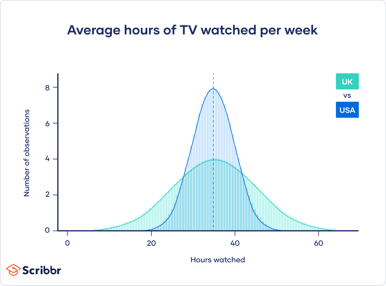
However, the British people surveyed had a wide variation in the number of hours watched, while the Americans all watched similar amounts.
Even though both groups have the same point estimate (average number of hours watched), the British estimate will have a wider confidence interval than the American estimate because there is more variation in the data.
Calculating a confidence interval: what you need to know
Most statistical programs will include the confidence interval of the estimate when you run a statistical test.
If you want to calculate a confidence interval on your own, you need to know:
- The point estimate you are constructing the confidence interval for
- The critical values for the test statistic
- The standard deviation of the sample
- The sample size
Once you know each of these components, you can calculate the confidence interval for your estimate by plugging them into the confidence interval formula that corresponds to your data.
Point estimate
The point estimate of your confidence interval will be whatever statistical estimate you are making (e.g., population mean, the difference between population means, proportions, variation among groups).
Finding the critical value
Critical values tell you how many standard deviations away from the mean you need to go in order to reach the desired confidence level for your confidence interval.
There are three steps to find the critical value.
- Choose your alpha (α) value.
The alpha value is the probability threshold for statistical significance. The most common alpha value is p = 0.05, but 0.1, 0.01, and even 0.001 are sometimes used. It’s best to look at the research papers published in your field to decide which alpha value to use.
- Decide if you need a one-tailed interval or a two-tailed interval.
You will most likely use a two-tailed interval unless you are doing a one-tailed t test.
For a two-tailed interval, divide your alpha by two to get the alpha value for the upper and lower tails.
- Look up the critical value that corresponds with the alpha value.
If your data follows a normal distribution, or if you have a large sample size (n > 30) that is approximately normally distributed, you can use the z distribution to find your critical values.
For a z statistic, some of the most common values are shown in this table:
| Confidence level | 90% | 95% | 99% |
|---|---|---|---|
| alpha for one-tailed CI | 0.1 | 0.05 | 0.01 |
| alpha for two-tailed CI | 0.05 | 0.025 | 0.005 |
| z statistic | 1.64 | 1.96 | 2.57 |
If you are using a small dataset (n ≤ 30) that is approximately normally distributed, use the t distribution instead.
The t distribution follows the same shape as the z distribution, but corrects for small sample sizes. For the t distribution, you need to know your degrees of freedom (sample size minus 1).
Check out this set of t tables to find your t statistic. We have included the confidence level and p values for both one-tailed and two-tailed tests to help you find the t value you need.
For normal distributions, like the t distribution and z distribution, the critical value is the same on either side of the mean.
For a two-tailed 95% confidence interval, the alpha value is 0.025, and the corresponding critical value is 1.96.
This means that to calculate the upper and lower bounds of the confidence interval, we can take the mean ±1.96 standard deviations from the mean.
Finding the standard deviation
Most statistical software will have a built-in function to calculate your standard deviation, but to find it by hand you can first find your sample variance, then take the square root to get the standard deviation.
- Find the sample variance
Sample variance is defined as the sum of squared differences from the mean, also known as the mean-squared-error (MSE):

To find the MSE, subtract your sample mean from each value in the dataset, square the resulting number, and divide that number by n − 1 (sample size minus 1).
Then add up all of these numbers to get your total sample variance (s2). For larger sample sets, it’s easiest to do this in Excel.
- Find the standard deviation.
The standard deviation of your estimate (s) is equal to the square root of the sample variance/sample error (s2):

- 10 for the GB estimate.
- 5 for the USA estimate.
Sample size
The sample size is the number of observations in your data set.
Confidence interval for the mean of normally-distributed data
Normally-distributed data forms a bell shape when plotted on a graph, with the sample mean in the middle and the rest of the data distributed fairly evenly on either side of the mean.
The confidence interval for data which follows a standard normal distribution is:

Where:
- CI = the confidence interval
- X̄ = the population mean
- Z* = the critical value of the z distribution
- σ = the population standard deviation
- √n = the square root of the population size
The confidence interval for the t distribution follows the same formula, but replaces the Z* with the t*.
In real life, you never know the true values for the population (unless you can do a complete census). Instead, we replace the population values with the values from our sample data, so the formula becomes:

Where:
- ˆx = the sample mean
- s = the sample standard deviation
To calculate the 95% confidence interval, we can simply plug the values into the formula.
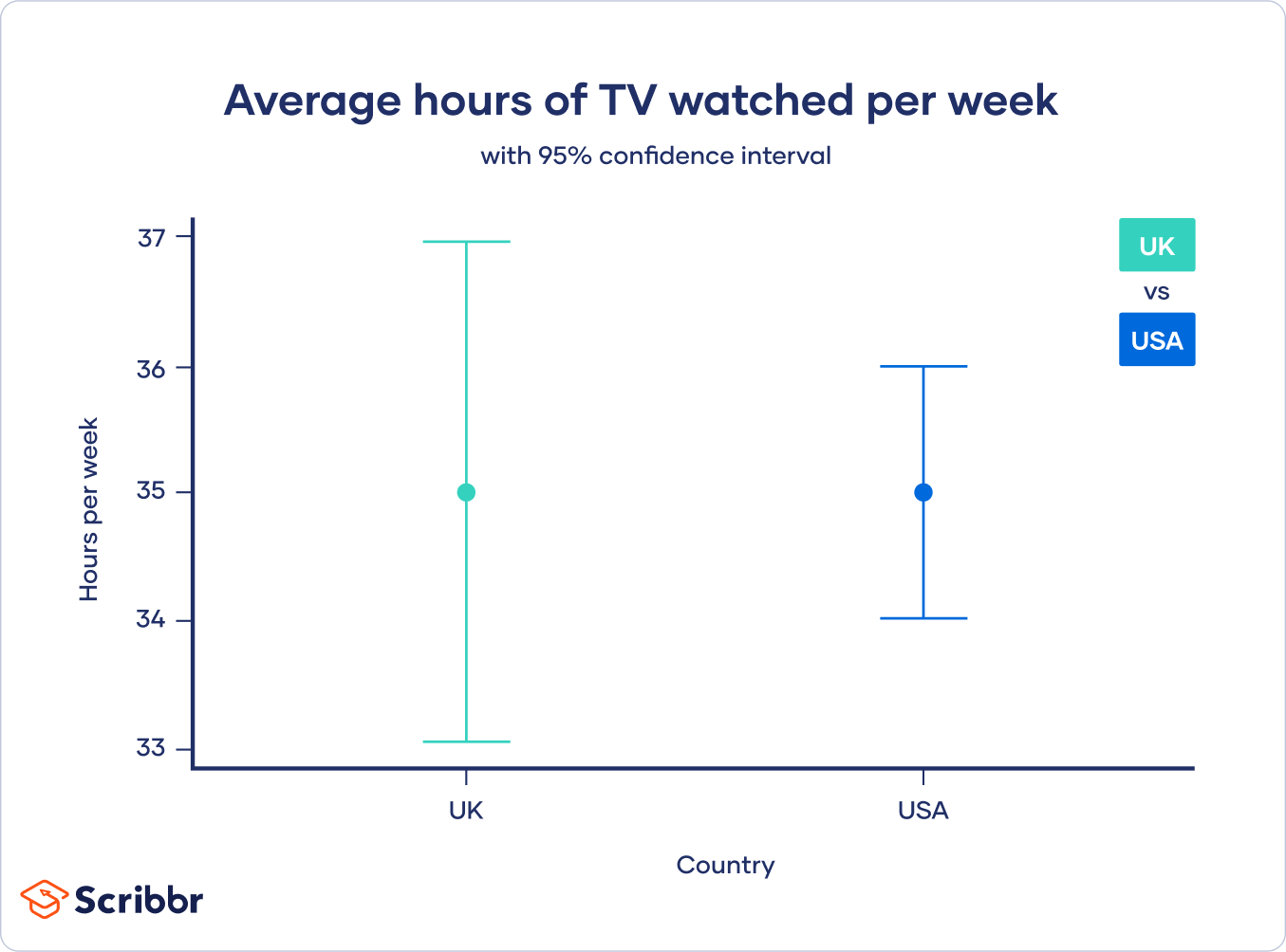
For the USA:

So for the USA, the lower and upper bounds of the 95% confidence interval are 34.02 and 35.98.
For GB:

So for the GB, the lower and upper bounds of the 95% confidence interval are 33.04 and 36.96.
Confidence interval for proportions
The confidence interval for a proportion follows the same pattern as the confidence interval for means, but place of the standard deviation you use the sample proportion times one minus the proportion:

Where:
- ˆp = the proportion in your sample (e.g. the proportion of respondents who said they watched any television at all)
- Z*= the critical value of the z distribution
- n = the sample size

Confidence interval for non-normally distributed data
To calculate a confidence interval around the mean of data that is not normally distributed, you have two choices:
- You can find a distribution that matches the shape of your data and use that distribution to calculate the confidence interval.
- You can perform a transformation on your data to make it fit a normal distribution, and then find the confidence interval for the transformed data.
Performing data transformations is very common in statistics, for example, when data follows a logarithmic curve but we want to use it alongside linear data. You just have to remember to do the reverse transformation on your data when you calculate the upper and lower bounds of the confidence interval.
Reporting confidence intervals
Confidence intervals are sometimes reported in papers, though researchers more often report the standard deviation of their estimate.
If you are asked to report the confidence interval, you should include the upper and lower bounds of the confidence interval.
One place that confidence intervals are frequently used is in graphs. When showing the differences between groups, or plotting a linear regression, researchers will often include the confidence interval to give a visual representation of the variation around the estimate.
Caution when using confidence intervals
Confidence intervals are sometimes interpreted as saying that the ‘true value’ of your estimate lies within the bounds of the confidence interval.
This is not the case. The confidence interval cannot tell you how likely it is that you found the true value of your statistical estimate because it is based on a sample, not on the whole population.
The confidence interval only tells you what range of values you can expect to find if you re-do your sampling or run your experiment again in the exact same way.
The more accurate your sampling plan, or the more realistic your experiment, the greater the chance that your confidence interval includes the true value of your estimate. But this accuracy is determined by your research methods, not by the statistics you do after you have collected the data!
Other interesting articles
If you want to know more about statistics, methodology, or research bias, make sure to check out some of our other articles with explanations and examples.
Statistics
Methodology
Frequently asked questions about confidence intervals
Cite this Scribbr article
If you want to cite this source, you can copy and paste the citation or click the “Cite this Scribbr article” button to automatically add the citation to our free Citation Generator.
Bevans, R. (2023, June 22). Understanding Confidence Intervals | Easy Examples & Formulas. Scribbr. Retrieved July 1, 2026, from https://www.scribbr.com/statistics/confidence-interval/
