Central Limit Theorem | Formula, Definition & Examples

Published on July 6, 2022 by Shaun Turney. Revised on June 22, 2023.

The central limit theorem states that if you take sufficiently large samples from a population, the samples’ means will be normally distributed, even if the population isn’t normally distributed.

What is the central limit theorem?
Central limit theorem formula
Sample size and the central limit theorem
Conditions of the central limit theorem
Importance of the central limit theorem
Central limit theorem examples
Practice questions
Other interesting articles
Frequently asked questions about the central limit theorem

What is the central limit theorem?

The central limit theorem relies on the concept of a sampling distribution, which is the probability distribution of a statistic for a large number of samples taken from a population.

Imagining an experiment may help you to understand sampling distributions:

Suppose that you draw a random sample from a population and calculate a statistic for the sample, such as the mean.
Now you draw another random sample of the same size, and again calculate the mean.
You repeat this process many times, and end up with a large number of means, one for each sample.

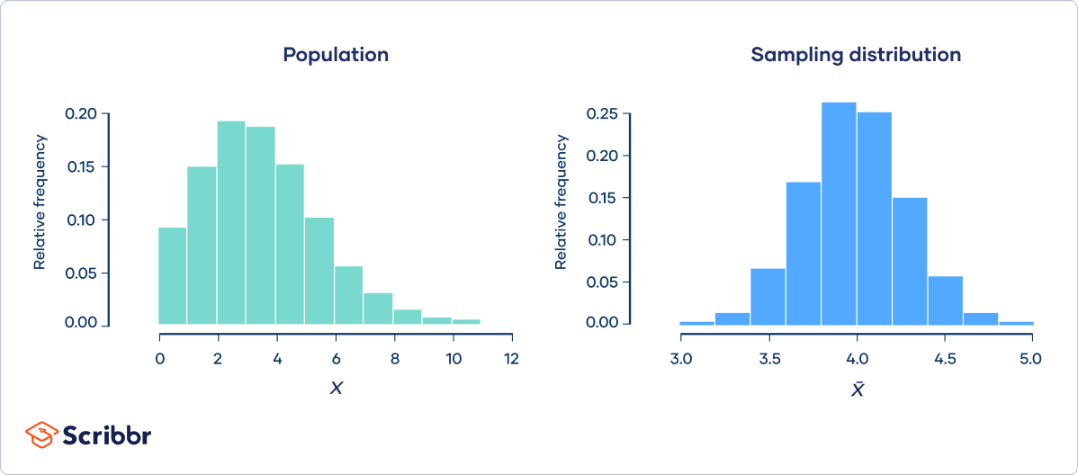
The distribution of the sample means is an example of a sampling distribution.

The central limit theorem says that the sampling distribution of the mean will always be normally distributed, as long as the sample size is large enough. Regardless of whether the population has a normal, Poisson, binomial, or any other distribution, the sampling distribution of the mean will be normal.

A normal distribution is a symmetrical, bell-shaped distribution, with increasingly fewer observations the further from the center of the distribution.

Receive feedback on language, structure, and formatting

Professional editors proofread and edit your paper by focusing on:

Academic style
Vague sentences
Grammar
Style consistency

See an example

Central limit theorem formula

Fortunately, you don’t need to actually repeatedly sample a population to know the shape of the sampling distribution. The parameters of the sampling distribution of the mean are determined by the parameters of the population:

The mean of the sampling distribution is the mean of the population.

$\begin{equation*}\mu_{\bar{x}}=\mu\end{equation*}$

The standard deviation of the sampling distribution is the standard deviation of the population divided by the square root of the sample size.

$\begin{equation*}\sigma_{\bar{x}} = \dfrac{\sigma}{\sqrt{n}}\end{equation*}$

We can describe the sampling distribution of the mean using this notation:

$\begin{equation*}\bar{X}\sim N (\mu,\dfrac{\sigma}{\sqrt{n}})\end{equation*}$

Where:

X̄ is the sampling distribution of the sample means
~ means “follows the distribution”
N is the normal distribution
µ is the mean of the population
σ is the standard deviation of the population
n is the sample size

Sample size and the central limit theorem

The sample size (n) is the number of observations drawn from the population for each sample. The sample size is the same for all samples.

The sample size affects the sampling distribution of the mean in two ways.

1. Sample size and normality

The larger the sample size, the more closely the sampling distribution will follow a normal distribution.

When the sample size is small, the sampling distribution of the mean is sometimes non-normal. That’s because the central limit theorem only holds true when the sample size is “sufficiently large.”

By convention, we consider a sample size of 30 to be “sufficiently large.”

When n < 30, the central limit theorem doesn’t apply. The sampling distribution will follow a similar distribution to the population. Therefore, the sampling distribution will only be normal if the population is normal.

When n ≥ 30, the central limit theorem applies. The sampling distribution will approximately follow a normal distribution.

2. Sample size and standard deviations

The sample size affects the standard deviation of the sampling distribution. Standard deviation is a measure of the variability or spread of the distribution (i.e., how wide or narrow it is).

When n is low, the standard deviation is high. There’s a lot of spread in the samples’ means because they aren’t precise estimates of the population’s mean.

When n is high, the standard deviation is low. There’s not much spread in the samples’ means because they’re precise estimates of the population’s mean.

Conditions of the central limit theorem

The central limit theorem states that the sampling distribution of the mean will always follow a normal distribution under the following conditions:

The sample size is sufficiently large. This condition is usually met if the sample size is n ≥ 30.

The samples are independent and identically distributed (i.i.d.) random variables. This condition is usually met if the sampling is random.

The population’s distribution has finite variance. Central limit theorem doesn’t apply to distributions with infinite variance, such as the Cauchy distribution. Most distributions have finite variance.

Here's why students love Scribbr's proofreading services

Discover proofreading & editing

Importance of the central limit theorem

The central limit theorem is one of the most fundamental statistical theorems. In fact, the “central” in “central limit theorem” refers to the importance of the theorem.

Note

Parametric tests, such as t tests, ANOVAs, and linear regression, have more statistical power than most non-parametric tests. Their statistical power comes from assumptions about populations’ distributions that are based on the central limit theorem.

Central limit theorem examples

Applying the central limit theorem to real distributions may help you to better understand how it works.

Continuous distribution

Suppose that you’re interested in the age that people retire in the United States. The population is all retired Americans, and the distribution of the population might look something like this:

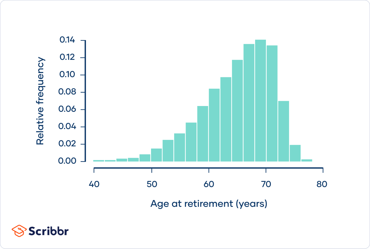
Age at retirement follows a left-skewed distribution. Most people retire within about five years of the mean retirement age of 65 years. However, there’s a “long tail” of people who retire much younger, such as at 50 or even 40 years old. The population has a standard deviation of 6 years.

Imagine that you take a small sample of the population. You randomly select five retirees and ask them what age they retired.

Example: Central limit theorem; sample of n = 5

The mean of the sample is an estimate of the population mean. It might not be a very precise estimate, since the sample size is only 5.

Example: Central limit theorem; mean of a small sample

mean = (68 + 73 + 70 + 62 + 63) / 5

mean = 67.2 years

Suppose that you repeat this procedure 10 times, taking samples of five retirees, and calculating the mean of each sample. This is a sampling distribution of the mean.

Example: Central limit theorem; means of 10 small samples

60.8

57.8

62.2

68.6

67.4

67.8

68.3

65.6

66.5

62.1

If you repeat the procedure many more times, a histogram of the sample means will look something like this:

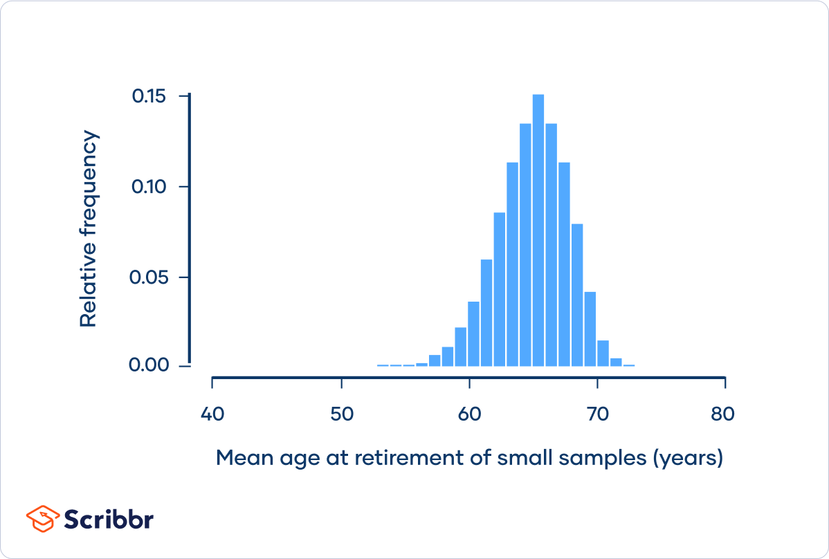
Although this sampling distribution is more normally distributed than the population, it still has a bit of a left skew.

Notice also that the spread of the sampling distribution is less than the spread of the population.

The central limit theorem says that the sampling distribution of the mean will always follow a normal distribution when the sample size is sufficiently large. This sampling distribution of the mean isn’t normally distributed because its sample size isn’t sufficiently large.

Now, imagine that you take a large sample of the population. You randomly select 50 retirees and ask them what age they retired.

Example: Central limit theorem; sample of n = 50

73	49	62	68	72	71	65	60	69	61
62	75	66	63	66	68	76	68	54	74
68	60	72	63	57	64	65	59	72	52
52	72	69	62	68	64	60	65	53	69
59	68	67	71	69	70	52	62	64	68

The mean of the sample is an estimate of the population mean. It’s a precise estimate, because the sample size is large.

Example: Central limit theorem; mean of a large sample

mean = 64.8 years

Again, you can repeat this procedure many more times, taking samples of fifty retirees, and calculating the mean of each sample:

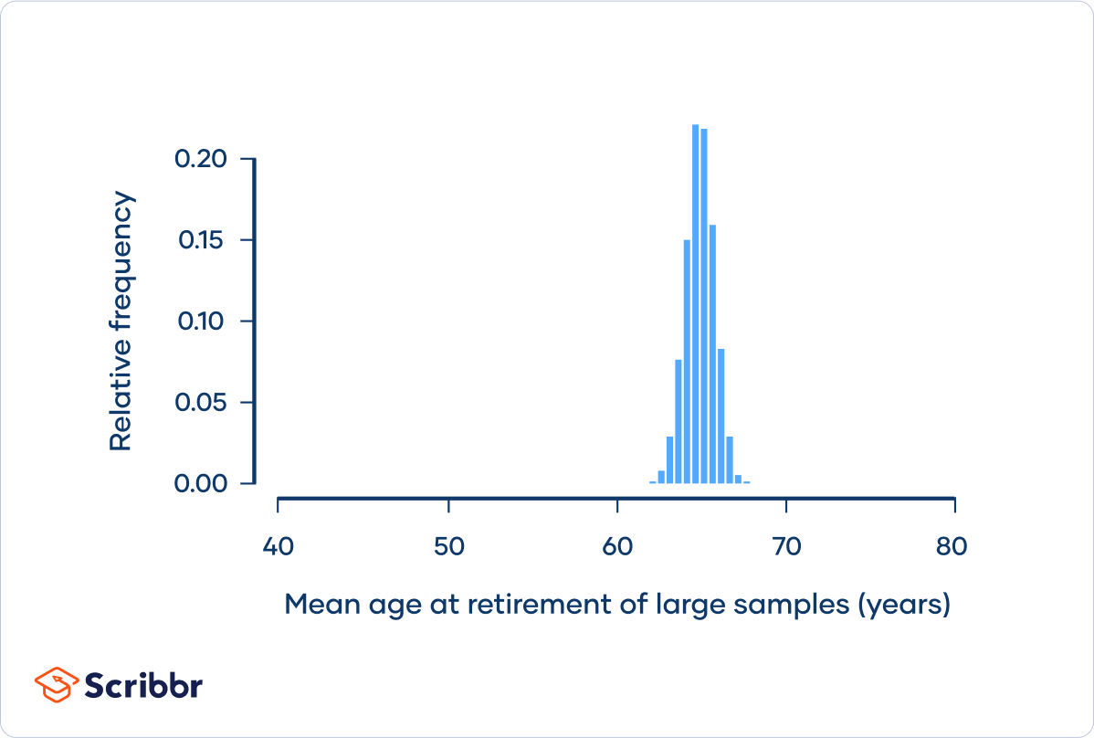
In the histogram, you can see that this sampling distribution is normally distributed, as predicted by the central limit theorem.

The standard deviation of this sampling distribution is 0.85 years, which is less than the spread of the small sample sampling distribution, and much less than the spread of the population. If you were to increase the sample size further, the spread would decrease even more.

We can use the central limit theorem formula to describe the sampling distribution:

$\bar{X} \sim N (\mu,\dfrac{\sigma}{\sqrt{n}})$

µ = 65

σ = 6

n = 50

$\bar{X} \sim N (65,\dfrac{6}{\sqrt{50}})$

$\bar{X} \sim N (65,0.85)$

Discrete distribution

Approximately 10% of people are left-handed. If we assign a value of 1 to left-handedness and a value of 0 to right-handedness, the probability distribution of left-handedness for the population of all humans looks like this:

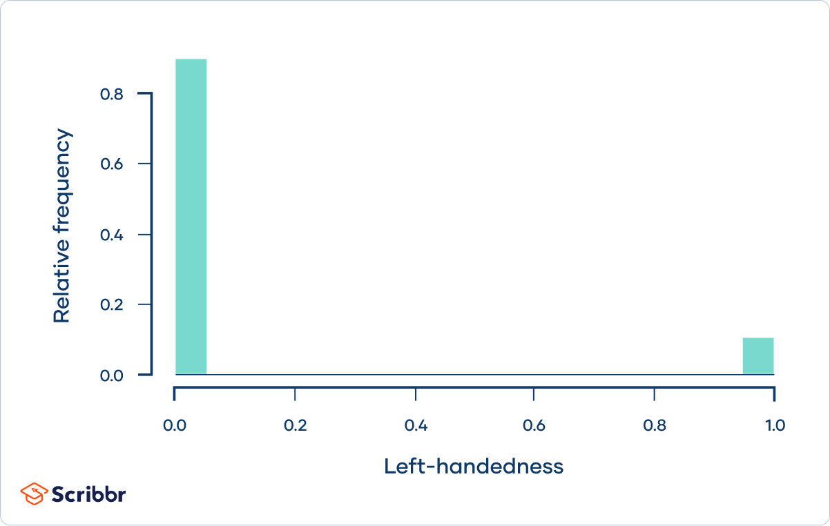
The population mean is the proportion of people who are left-handed (0.1). The population standard deviation is 0.3.

Imagine that you take a random sample of five people and ask them whether they’re left-handed.

Example: Central limit theorem; sample of n = 5

The mean of the sample is an estimate of the population mean. It might not be a very precise estimate, since the sample size is only 5.

Example: Central limit theorem; mean of a small sample

mean = (0 + 0 + 0 + 1 + 0) / 5

mean = 0.2

Imagine you repeat this process 10 times, randomly sampling five people and calculating the mean of the sample. This is a sampling distribution of the mean.

Example: Central limit theorem; means of 10 small samples

0.4

0.2

0.4

If you repeat this process many more times, the distribution will look something like this:

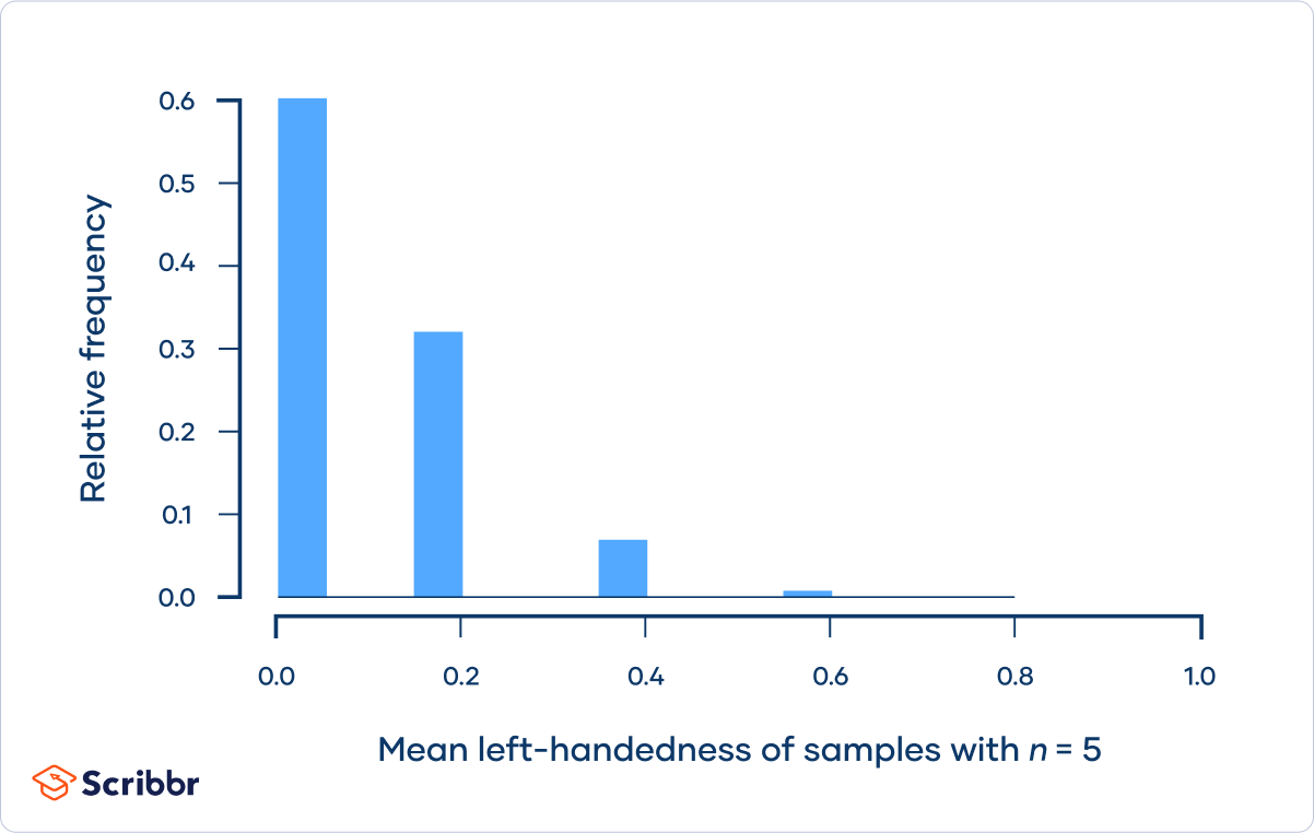
The sampling distribution isn’t normally distributed because the sample size isn’t sufficiently large for the central limit theorem to apply.

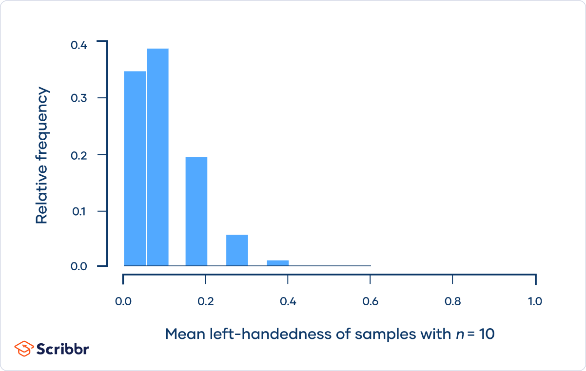
As the sample size increases, the sampling distribution looks increasingly similar to a normal distribution, and the spread decreases:

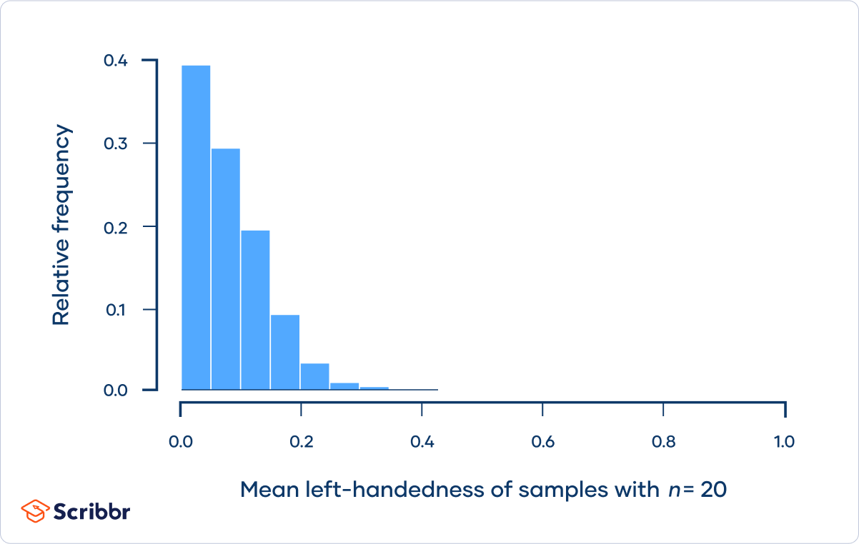
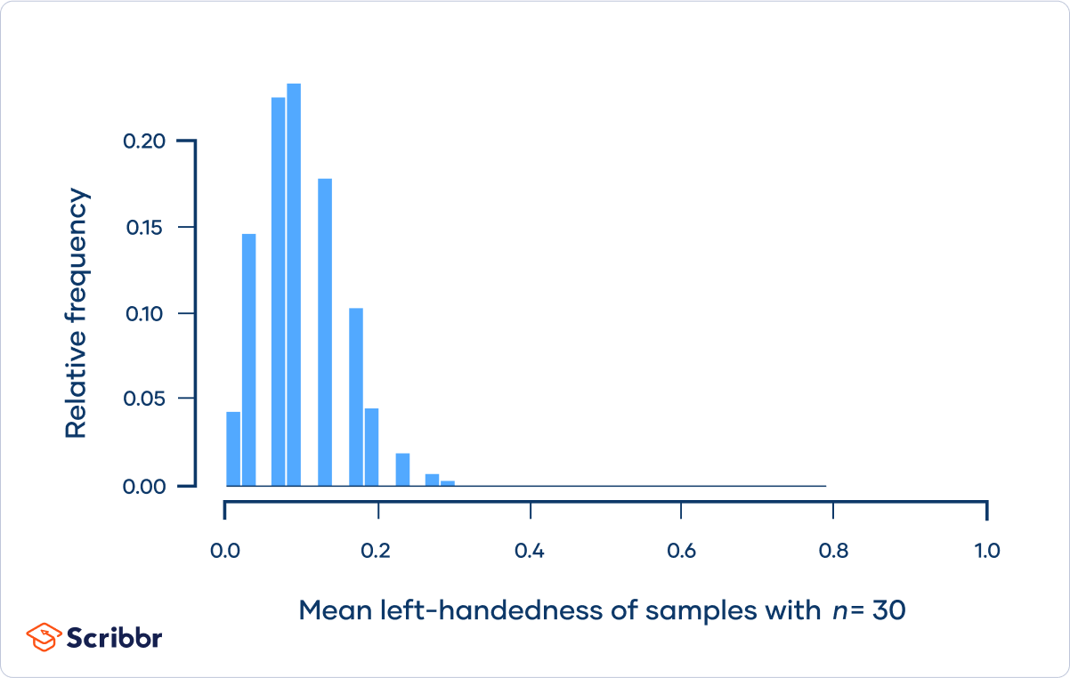
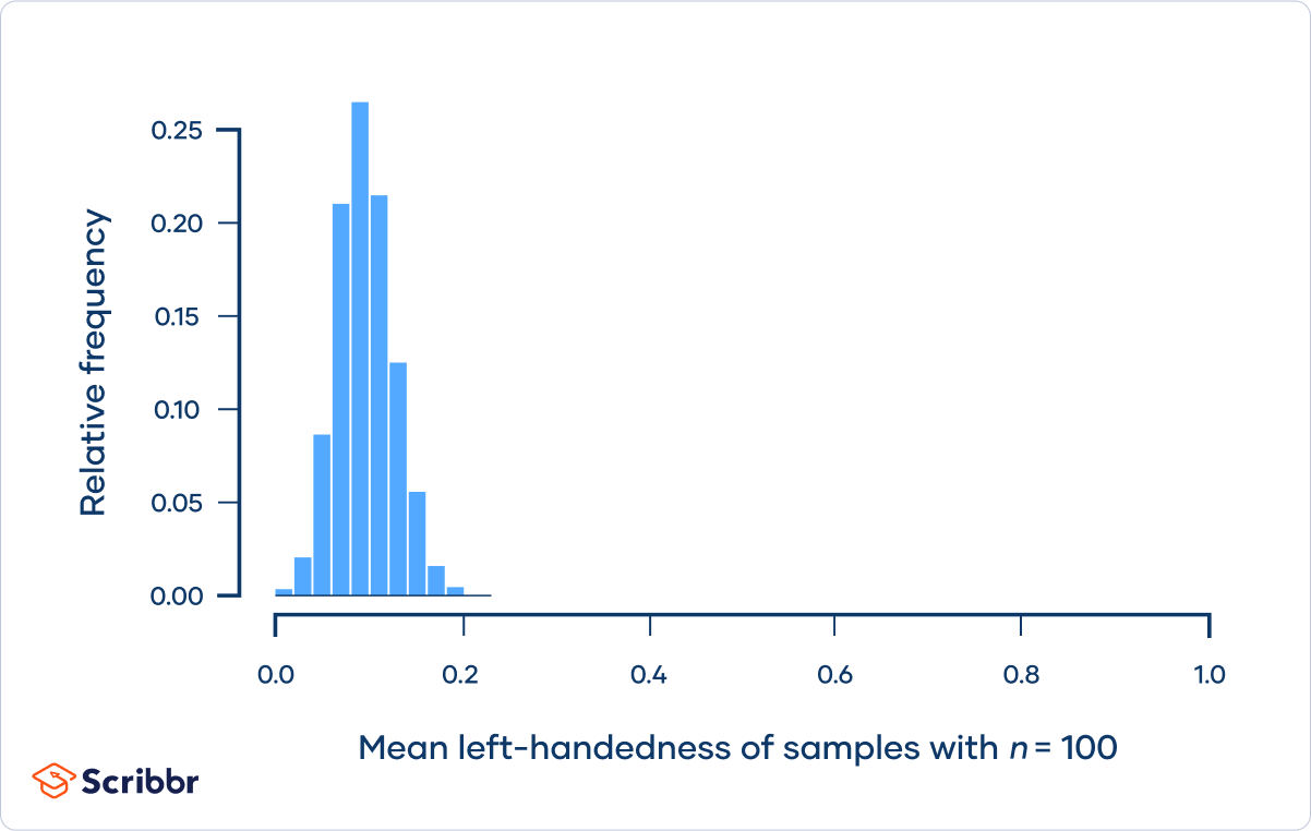
The sampling distribution of the mean for samples with n = 30 approaches normality. When the sample size is increased further to n = 100, the sampling distribution follows a normal distribution.

We can use the central limit theorem formula to describe the sampling distribution for n = 100.

$\bar{X} \sim N (\mu,\dfrac{\sigma}{\sqrt{n}})$

µ = 0.1

σ = 0.3

n = 100

$\bar{X} \sim N (0.1,\dfrac{0.3}{\sqrt{100}})$

$\bar{X} \sim N (0.1,0.03)$

Practice questions

Frequently asked questions about the central limit theorem

What is a normal distribution?: In a normal distribution, data are symmetrically distributed with no skew. Most values cluster around a central region, with values tapering off as they go further away from the center.

The measures of central tendency (mean, mode, and median) are exactly the same in a normal distribution.
What are the three types of skewness?: The three types of skewness are:

Right skew (also called positive skew). A right-skewed distribution is longer on the right side of its peak than on its left.

Left skew (also called negative skew). A left-skewed distribution is longer on the left side of its peak than on its right.

Zero skew. It is symmetrical and its left and right sides are mirror images.
Why are samples used in research?: Samples are used to make inferences about populations. Samples are easier to collect data from because they are practical, cost-effective, convenient, and manageable.

Cite this Scribbr article

If you want to cite this source, you can copy and paste the citation or click the “Cite this Scribbr article” button to automatically add the citation to our free Citation Generator.

Turney, S. (2023, June 22). Central Limit Theorem | Formula, Definition & Examples. Scribbr. Retrieved April 16, 2024, from https://www.scribbr.com/statistics/central-limit-theorem/

Cite this article

Is this article helpful?

You have already voted. Thanks :-) Your vote is saved :-) Processing your vote...

Shaun Turney

During his MSc and PhD, Shaun learned how to apply scientific and statistical methods to his research in ecology. Now he loves to teach students how to collect and analyze data for their own theses and research projects.

Have a language expert improve your writing

Run a free plagiarism check in 10 minutes

Generate accurate citations for free

Proofreading & Editing

AI Proofreader

Plagiarism Checker

Citation Generator

Paraphraser

Grammar Checker

Central Limit Theorem | Formula, Definition & Examples

Table of contents

What is the central limit theorem?

Receive feedback on language, structure, and formatting

Central limit theorem formula