Normal Distribution | Examples, Formulas, & Uses
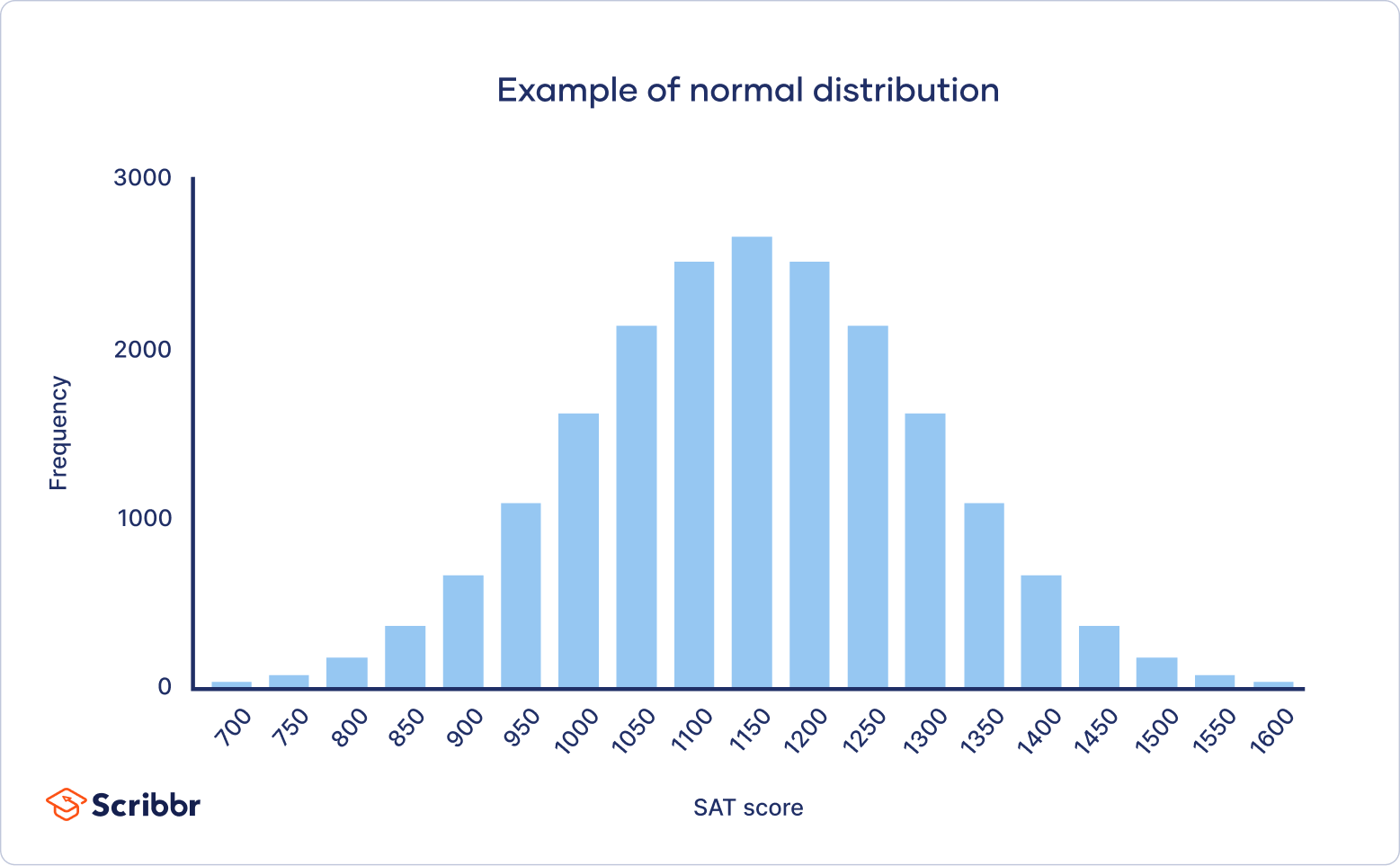
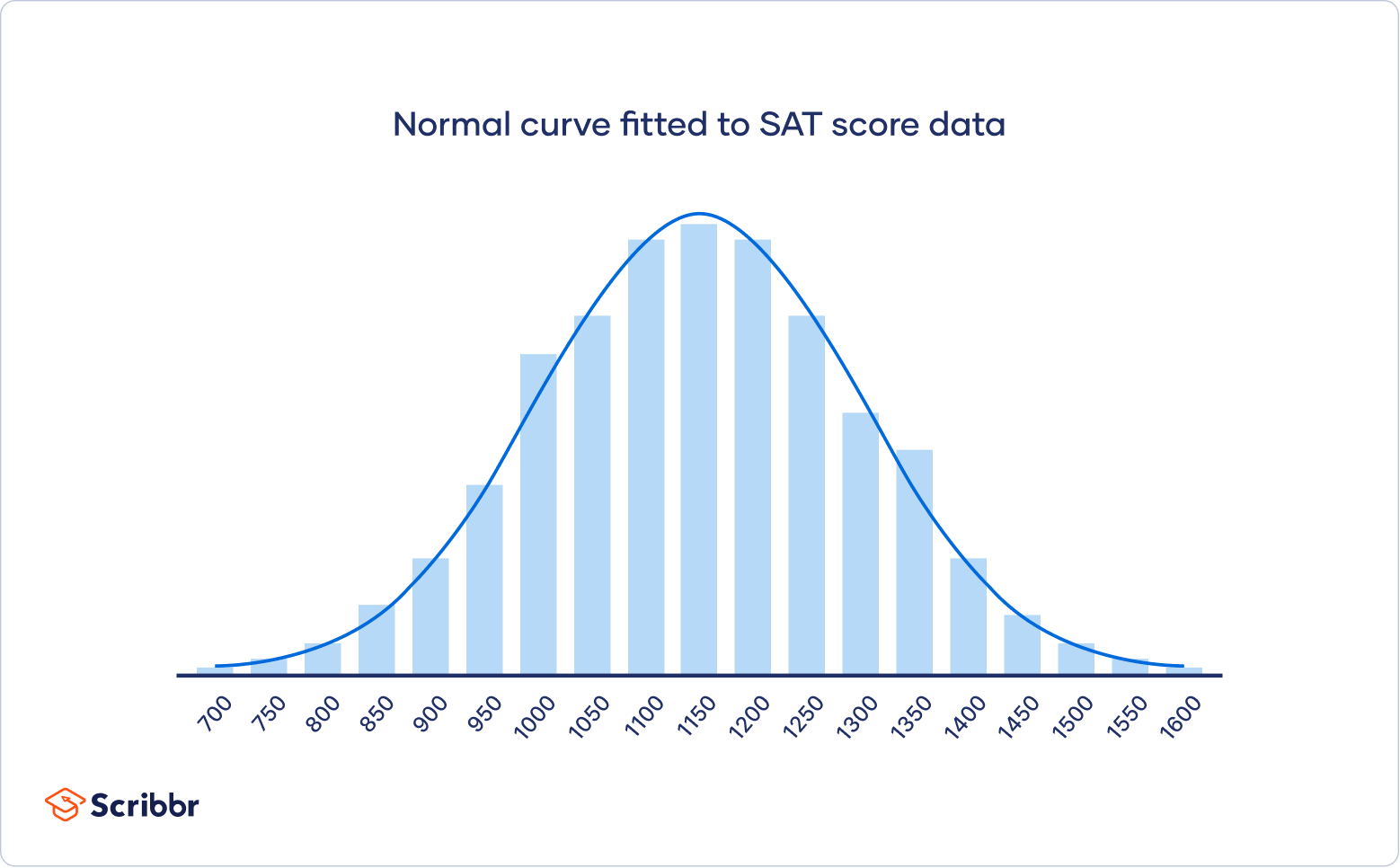
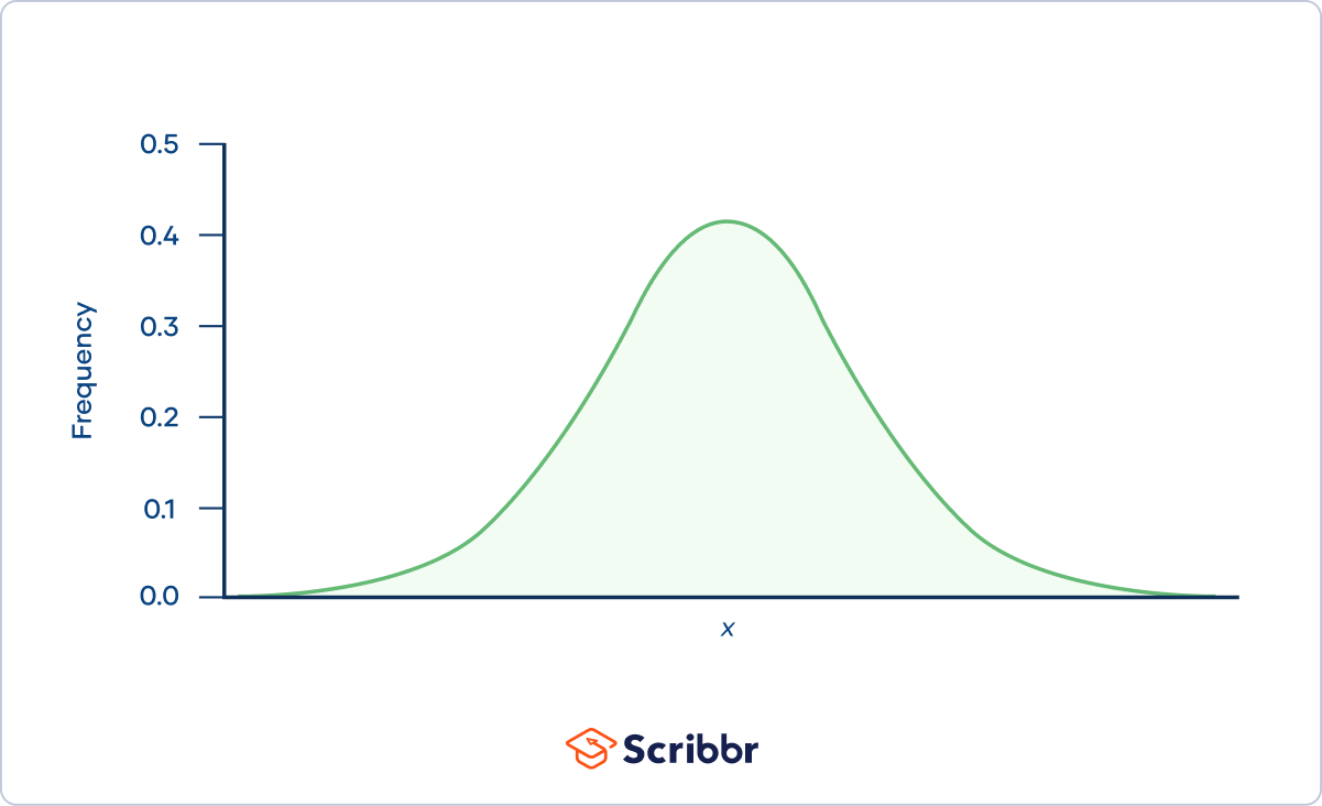
In a normal distribution, data is symmetrically distributed with no skew. When plotted on a graph, the data follows a bell shape, with most values clustering around a central region and tapering off as they go further away from the center.
Normal distributions are also called Gaussian distributions or bell curves because of their shape.
Why do normal distributions matter?
All kinds of variables in natural and social sciences are normally or approximately normally distributed. Height, birth weight, reading ability, job satisfaction, or SAT scores are just a few examples of such variables.
Because normally distributed variables are so common, many statistical tests are designed for normally distributed populations.
Understanding the properties of normal distributions means you can use inferential statistics to compare different groups and make estimates about populations using samples.
What are the properties of normal distributions?
Normal distributions have key characteristics that are easy to spot in graphs:
- The mean, median and mode are exactly the same.
- The distribution is symmetric about the mean—half the values fall below the mean and half above the mean.
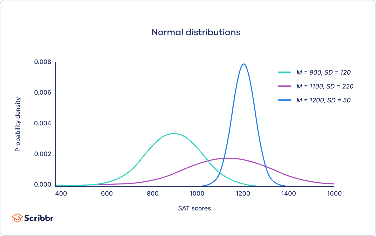
- The distribution can be described by two values: the mean and the standard deviation.
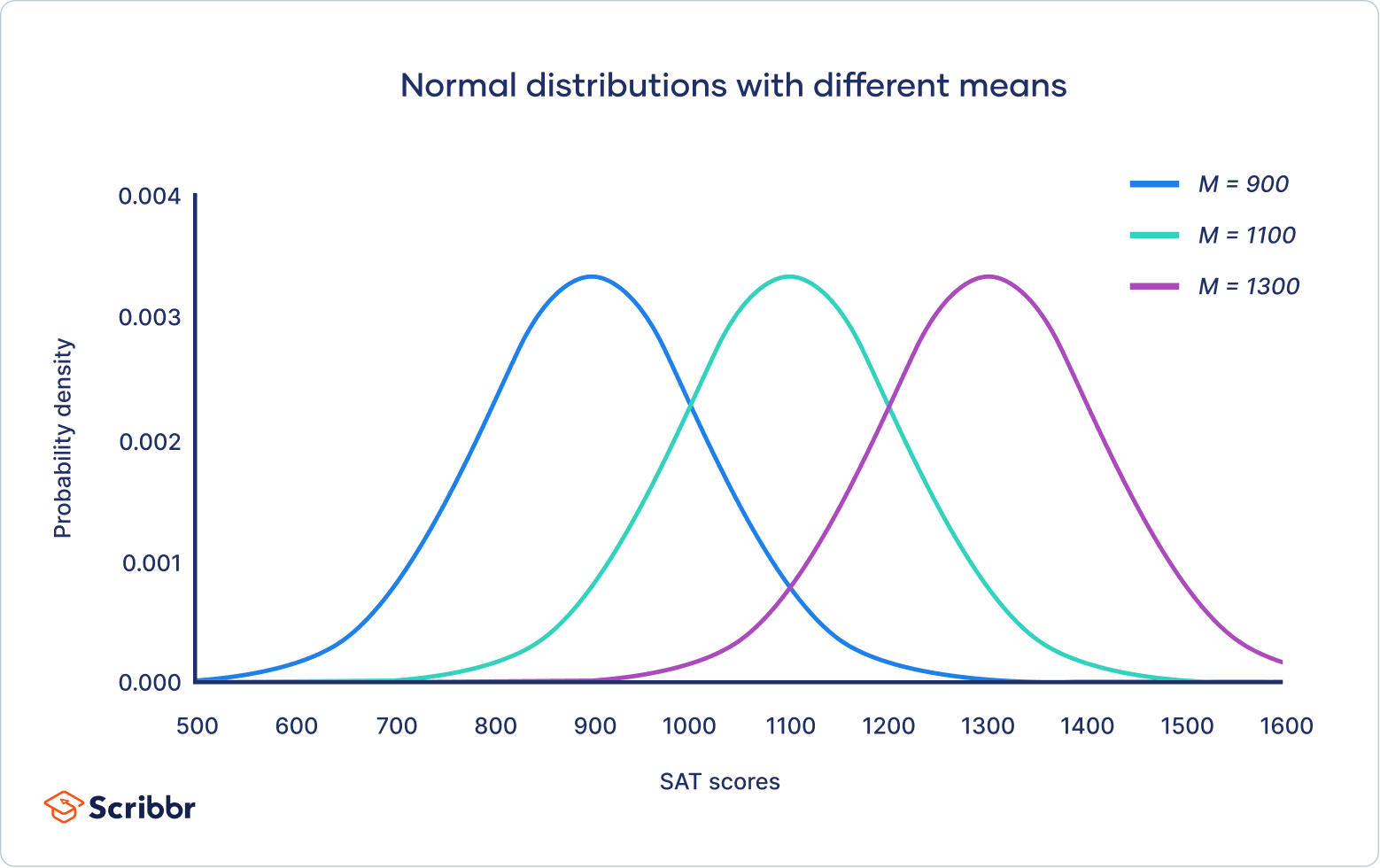
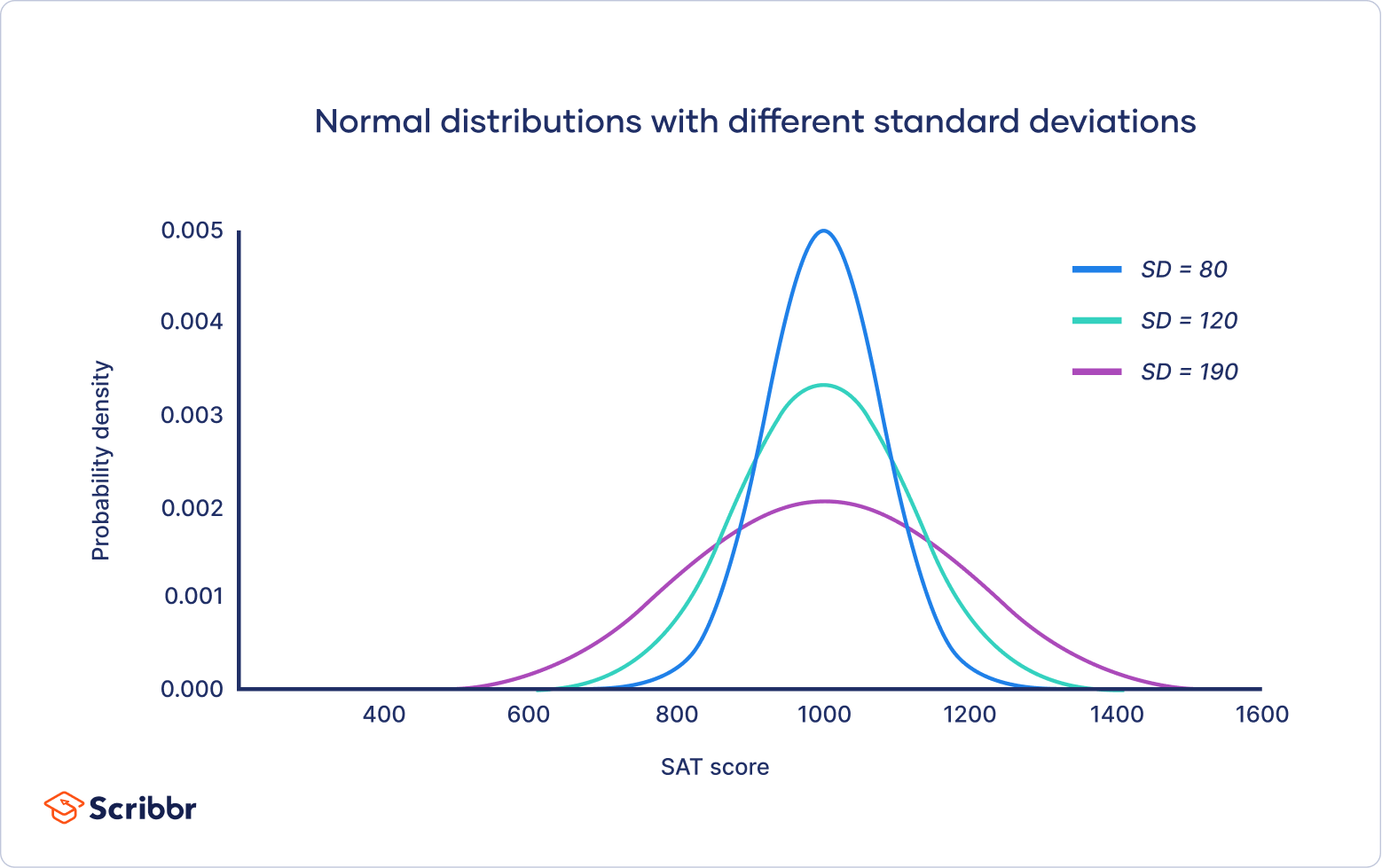
The mean is the location parameter while the standard deviation is the scale parameter.
The mean determines where the peak of the curve is centered. Increasing the mean moves the curve right, while decreasing it moves the curve left.
The standard deviation stretches or squeezes the curve. A small standard deviation results in a narrow curve, while a large standard deviation leads to a wide curve.
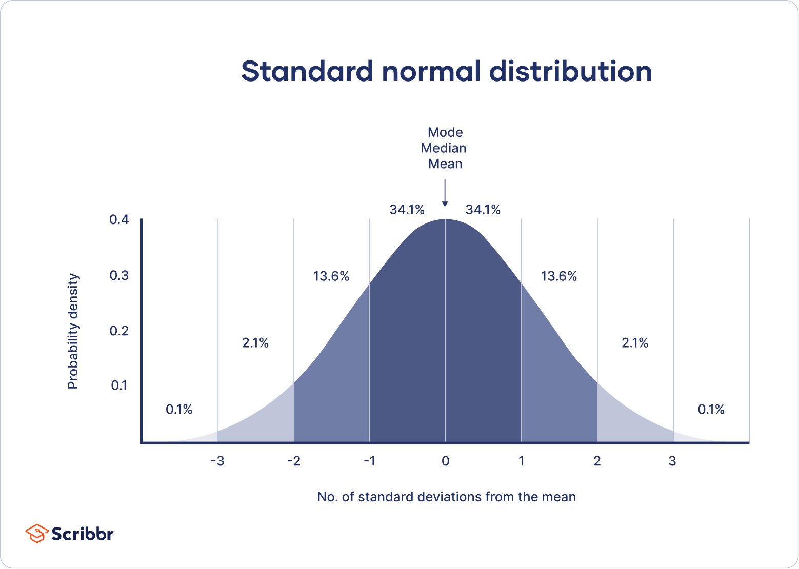
Empirical rule
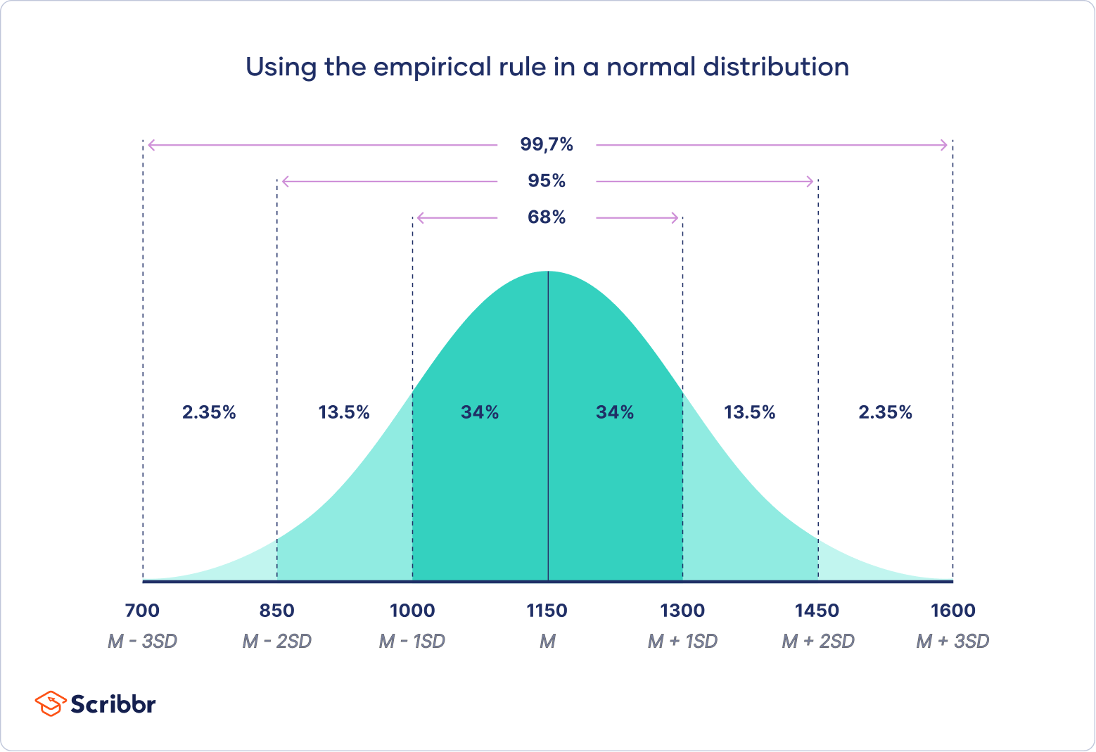
The empirical rule, or the 68-95-99.7 rule, tells you where most of your values lie in a normal distribution:
- Around 68% of values are within 1 standard deviation from the mean.
- Around 95% of values are within 2 standard deviations from the mean.
- Around 99.7% of values are within 3 standard deviations from the mean.
Following the empirical rule:
- Around 68% of scores are between 1,000 and 1,300, 1 standard deviation above and below the mean.
- Around 95% of scores are between 850 and 1,450, 2 standard deviations above and below the mean.
- Around 99.7% of scores are between 700 and 1,600, 3 standard deviations above and below the mean.
The empirical rule is a quick way to get an overview of your data and check for any outliers or extreme values that don’t follow this pattern.
If data from small samples do not closely follow this pattern, then other distributions like the t-distribution may be more appropriate. Once you identify the distribution of your variable, you can apply appropriate statistical tests.
Central limit theorem
The central limit theorem is the basis for how normal distributions work in statistics.
In research, to get a good idea of a population mean, ideally you’d collect data from multiple random samples within the population. A sampling distribution of the mean is the distribution of the means of these different samples.
The central limit theorem shows the following:
- Law of Large Numbers: As you increase sample size (or the number of samples), then the sample mean will approach the population mean.
- With multiple large samples, the sampling distribution of the mean is normally distributed, even if your original variable is not normally distributed.
Parametric statistical tests typically assume that samples come from normally distributed populations, but the central limit theorem means that this assumption isn’t necessary to meet when you have a large enough sample.
You can use parametric tests for large samples from populations with any kind of distribution as long as other important assumptions are met. A sample size of 30 or more is generally considered large.
For small samples, the assumption of normality is important because the sampling distribution of the mean isn’t known. For accurate results, you have to be sure that the population is normally distributed before you can use parametric tests with small samples.
Here's why students love Scribbr's proofreading services
Formula of the normal curve
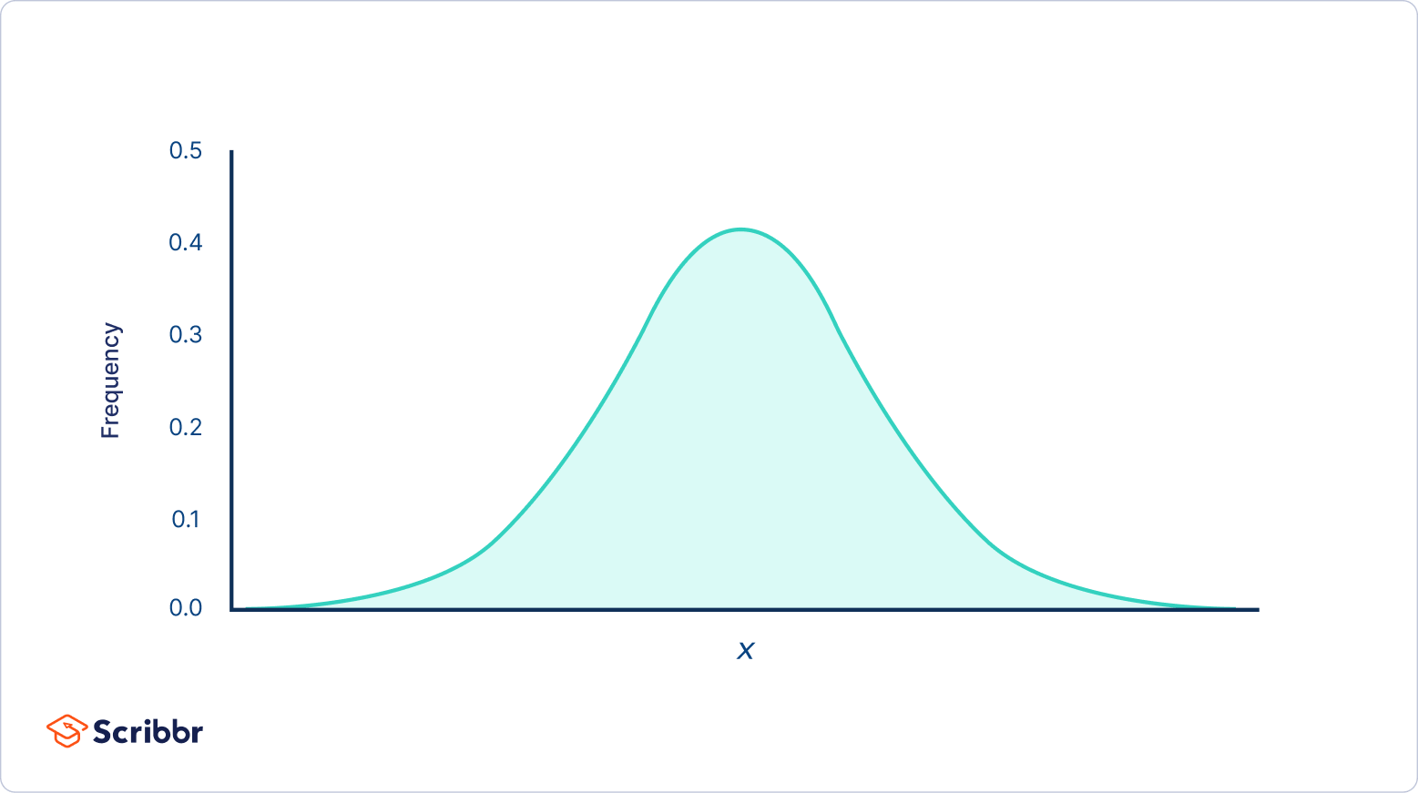
Once you have the mean and standard deviation of a normal distribution, you can fit a normal curve to your data using a probability density function.
In a probability density function, the area under the curve tells you probability. The normal distribution is a probability distribution, so the total area under the curve is always 1 or 100%.
The formula for the normal probability density function looks fairly complicated. But to use it, you only need to know the population mean and standard deviation.
For any value of x, you can plug in the mean and standard deviation into the formula to find the probability density of the variable taking on that value of x.
| Normal probability density formula | Explanation |
|---|---|
 |
|
On your graph of the probability density function, the probability is the shaded area under the curve that lies to the right of where your SAT scores equal 1380.
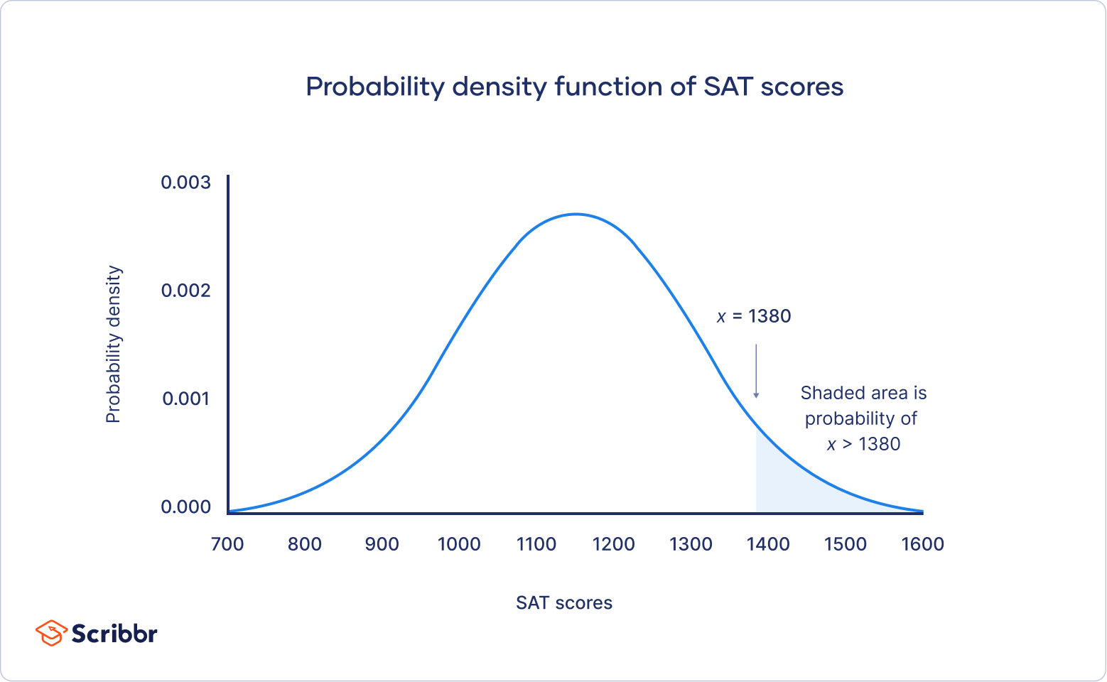
You can find the probability value of this score using the standard normal distribution.
What is the standard normal distribution?
The standard normal distribution, also called the z-distribution, is a special normal distribution where the mean is 0 and the standard deviation is 1.
Every normal distribution is a version of the standard normal distribution that’s been stretched or squeezed and moved horizontally right or left.
While individual observations from normal distributions are referred to as x, they are referred to as z in the z-distribution. Every normal distribution can be converted to the standard normal distribution by turning the individual values into z-scores.
Z-scores tell you how many standard deviations away from the mean each value lies.
You only need to know the mean and standard deviation of your distribution to find the z-score of a value.
| Z-score Formula | Explanation |
|---|---|
 |
|
We convert normal distributions into the standard normal distribution for several reasons:
- To find the probability of observations in a distribution falling above or below a given value.
- To find the probability that a sample mean significantly differs from a known population mean.
- To compare scores on different distributions with different means and standard deviations.
Finding probability using the z-distribution
Each z-score is associated with a probability, or p-value, that tells you the likelihood of values below that z-score occurring. If you convert an individual value into a z-score, you can then find the probability of all values up to that value occurring in a normal distribution.
The mean of our distribution is 1150, and the standard deviation is 150. The z-score tells you how many standard deviations away 1380 is from the mean.
| Formula | Calculation |
|---|---|
|
  |
For a z-score of 1.53, the p-value is 0.937. This is the probability of SAT scores being 1380 or less (93.7%), and it’s the area under the curve left of the shaded area.
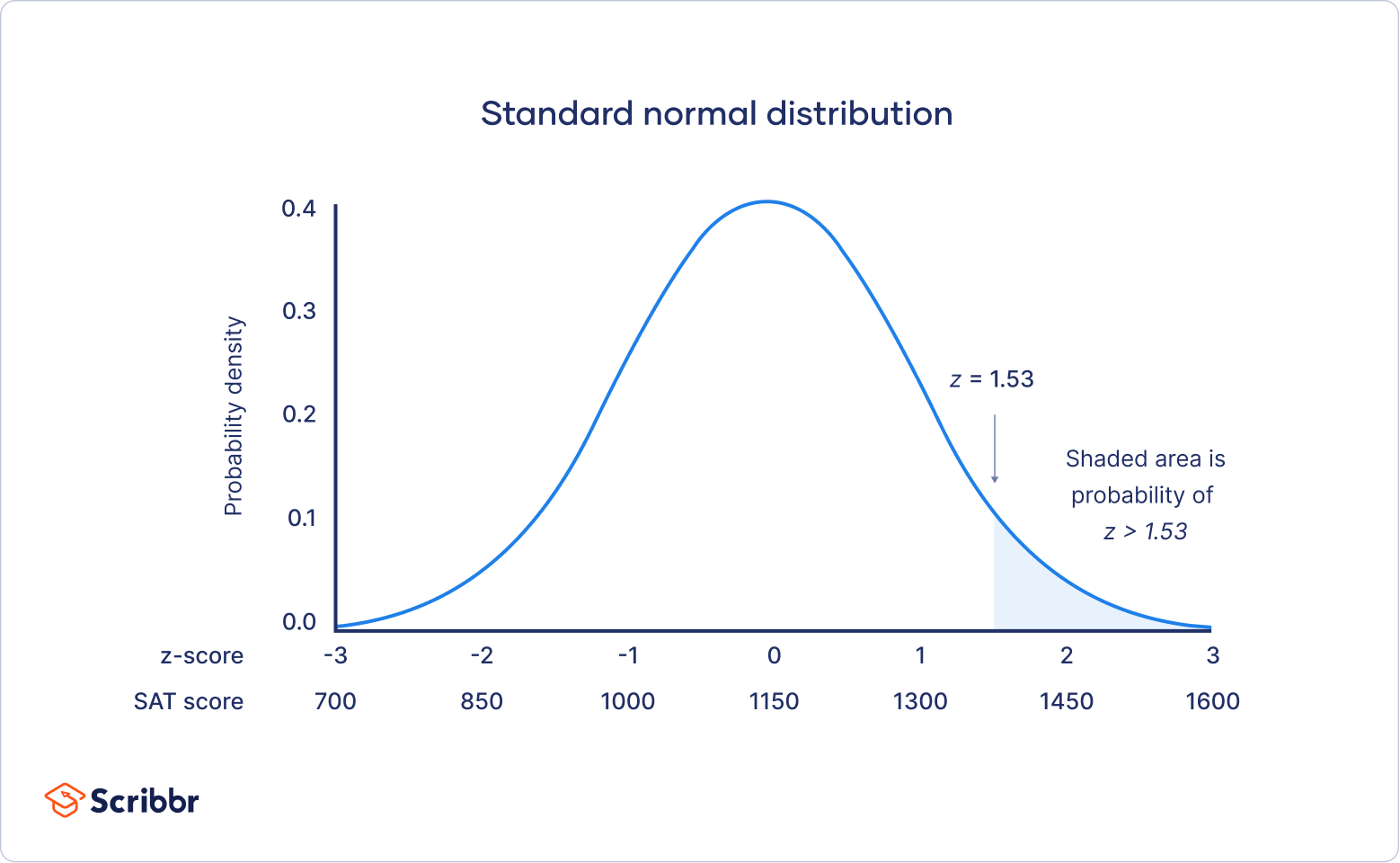
To find the shaded area, you take away 0.937 from 1, which is the total area under the curve.
Probability of x > 1380 = 1 – 0.937 = 0.063
That means it is likely that only 6.3% of SAT scores in your sample exceed 1380.
Other interesting articles
If you want to know more about statistics, methodology, or research bias, make sure to check out some of our other articles with explanations and examples.
Statistics
Methodology
Frequently asked questions about normal distributions
Cite this Scribbr article
If you want to cite this source, you can copy and paste the citation or click the “Cite this Scribbr article” button to automatically add the citation to our free Citation Generator.
Bhandari, P. (2023, June 21). Normal Distribution | Examples, Formulas, & Uses. Scribbr. Retrieved July 9, 2026, from https://www.scribbr.com/statistics/normal-distribution/