Simple Linear Regression | An Easy Introduction & Examples
Simple linear regression is used to estimate the relationship between two quantitative variables. You can use simple linear regression when you want to know:
- How strong the relationship is between two variables (e.g., the relationship between rainfall and soil erosion).
- The value of the dependent variable at a certain value of the independent variable (e.g., the amount of soil erosion at a certain level of rainfall).
Regression models describe the relationship between variables by fitting a line to the observed data. Linear regression models use a straight line, while logistic and nonlinear regression models use a curved line. Regression allows you to estimate how a dependent variable changes as the independent variable(s) change.
Your independent variable (income) and dependent variable (happiness) are both quantitative, so you can do a regression analysis to see if there is a linear relationship between them.
If you have more than one independent variable, use multiple linear regression instead.
Assumptions of simple linear regression
Simple linear regression is a parametric test, meaning that it makes certain assumptions about the data. These assumptions are:
- Homogeneity of variance (homoscedasticity): the size of the error in our prediction doesn’t change significantly across the values of the independent variable.
- Independence of observations: the observations in the dataset were collected using statistically valid sampling methods, and there are no hidden relationships among observations.
- Normality: The data follows a normal distribution.
Linear regression makes one additional assumption:
- The relationship between the independent and dependent variable is linear: the line of best fit through the data points is a straight line (rather than a curve or some sort of grouping factor).
If your data do not meet the assumptions of homoscedasticity or normality, you may be able to use a nonparametric test instead, such as the Spearman rank test.
If your data violate the assumption of independence of observations (e.g., if observations are repeated over time), you may be able to perform a linear mixed-effects model that accounts for the additional structure in the data.
How to perform a simple linear regression
Simple linear regression formula
The formula for a simple linear regression is:

- y is the predicted value of the dependent variable (y) for any given value of the independent variable (x).
- B0 is the intercept, the predicted value of y when the x is 0.
- B1 is the regression coefficient – how much we expect y to change as x increases.
- x is the independent variable ( the variable we expect is influencing y).
- e is the error of the estimate, or how much variation there is in our estimate of the regression coefficient.
Linear regression finds the line of best fit line through your data by searching for the regression coefficient (B1) that minimizes the total error (e) of the model.
While you can perform a linear regression by hand, this is a tedious process, so most people use statistical programs to help them quickly analyze the data.
Simple linear regression in R
R is a free, powerful, and widely-used statistical program. Download the dataset to try it yourself using our income and happiness example.
Dataset for simple linear regression (.csv)
Load the income.data dataset into your R environment, and then run the following command to generate a linear model describing the relationship between income and happiness:
income.happiness.lm <- lm(happiness ~ income, data = income.data)This code takes the data you have collected data = income.data and calculates the effect that the independent variable income has on the dependent variable happiness using the equation for the linear model: lm().
To learn more, follow our full step-by-step guide to linear regression in R.
Interpreting the results
To view the results of the model, you can use the summary() function in R:
summary(income.happiness.lm)This function takes the most important parameters from the linear model and puts them into a table, which looks like this:
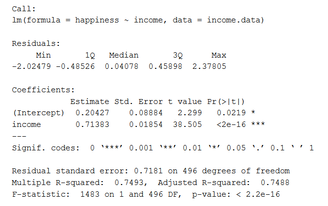
This output table first repeats the formula that was used to generate the results (‘Call’), then summarizes the model residuals (‘Residuals’), which give an idea of how well the model fits the real data.
Next is the ‘Coefficients’ table. The first row gives the estimates of the y-intercept, and the second row gives the regression coefficient of the model.
Row 1 of the table is labeled (Intercept). This is the y-intercept of the regression equation, with a value of 0.20. You can plug this into your regression equation if you want to predict happiness values across the range of income that you have observed:
The next row in the ‘Coefficients’ table is income. This is the row that describes the estimated effect of income on reported happiness:
The Estimate column is the estimated effect, also called the regression coefficient or r2 value. The number in the table (0.713) tells us that for every one unit increase in income (where one unit of income = 10,000) there is a corresponding 0.71-unit increase in reported happiness (where happiness is a scale of 1 to 10).
The Std. Error column displays the standard error of the estimate. This number shows how much variation there is in our estimate of the relationship between income and happiness.
The t value column displays the test statistic. Unless you specify otherwise, the test statistic used in linear regression is the t value from a two-sided t test. The larger the test statistic, the less likely it is that our results occurred by chance.
The Pr(>| t |) column shows the p value. This number tells us how likely we are to see the estimated effect of income on happiness if the null hypothesis of no effect were true.
Because the p value is so low (p < 0.001), we can reject the null hypothesis and conclude that income has a statistically significant effect on happiness.
The last three lines of the model summary are statistics about the model as a whole. The most important thing to notice here is the p value of the model. Here it is significant (p < 0.001), which means that this model is a good fit for the observed data.
Presenting the results
When reporting your results, include the estimated effect (i.e. the regression coefficient), standard error of the estimate, and the p value. You should also interpret your numbers to make it clear to your readers what your regression coefficient means:
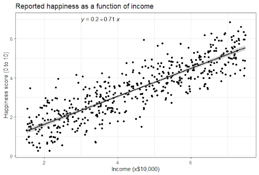
It can also be helpful to include a graph with your results. For a simple linear regression, you can simply plot the observations on the x and y axis and then include the regression line and regression function:
Here's why students love Scribbr's proofreading services
Can you predict values outside the range of your data?
No! We often say that regression models can be used to predict the value of the dependent variable at certain values of the independent variable. However, this is only true for the range of values where we have actually measured the response.
We can use our income and happiness regression analysis as an example. Between 15,000 and 75,000, we found an r2 of 0.73 ± 0.0193. But what if we did a second survey of people making between 75,000 and 150,000?
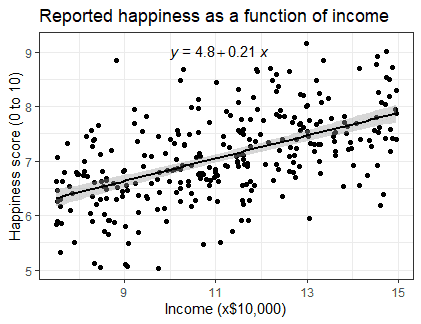
The r2 for the relationship between income and happiness is now 0.21, or a 0.21-unit increase in reported happiness for every 10,000 increase in income. While the relationship is still statistically significant (p<0.001), the slope is much smaller than before.
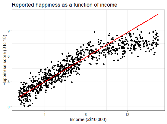
What if we hadn’t measured this group, and instead extrapolated the line from the 15–75k incomes to the 70–150k incomes?
You can see that if we simply extrapolated from the 15–75k income data, we would overestimate the happiness of people in the 75–150k income range.
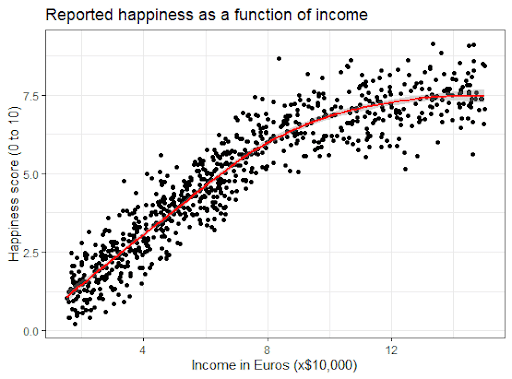
If we instead fit a curve to the data, it seems to fit the actual pattern much better.
It looks as though happiness actually levels off at higher incomes, so we can’t use the same regression line we calculated from our lower-income data to predict happiness at higher levels of income.
Even when you see a strong pattern in your data, you can’t know for certain whether that pattern continues beyond the range of values you have actually measured. Therefore, it’s important to avoid extrapolating beyond what the data actually tell you.
Other interesting articles
If you want to know more about statistics, methodology, or research bias, make sure to check out some of our other articles with explanations and examples.
Statistics
Methodology
Frequently asked questions about simple linear regression
Cite this Scribbr article
If you want to cite this source, you can copy and paste the citation or click the “Cite this Scribbr article” button to automatically add the citation to our free Citation Generator.
Bevans, R. (2023, June 22). Simple Linear Regression | An Easy Introduction & Examples. Scribbr. Retrieved July 15, 2026, from https://www.scribbr.com/statistics/simple-linear-regression/
