The Beginner's Guide to Statistical Analysis | 5 Steps & Examples
Statistical analysis means investigating trends, patterns, and relationships using quantitative data. It is an important research tool used by scientists, governments, businesses, and other organizations.
To draw valid conclusions, statistical analysis requires careful planning from the very start of the research process. You need to specify your hypotheses and make decisions about your research design, sample size, and sampling procedure.
After collecting data from your sample, you can organize and summarize the data using descriptive statistics. Then, you can use inferential statistics to formally test hypotheses and make estimates about the population. Finally, you can interpret and generalize your findings.
This article is a practical introduction to statistical analysis for students and researchers. We’ll walk you through the steps using two research examples. The first investigates a potential cause-and-effect relationship, while the second investigates a potential correlation between variables.
Step 1: Write your hypotheses and plan your research design
To collect valid data for statistical analysis, you first need to specify your hypotheses and plan out your research design.
Writing statistical hypotheses
The goal of research is often to investigate a relationship between variables within a population. You start with a prediction, and use statistical analysis to test that prediction.
A statistical hypothesis is a formal way of writing a prediction about a population. Every research prediction is rephrased into null and alternative hypotheses that can be tested using sample data.
While the null hypothesis always predicts no effect or no relationship between variables, the alternative hypothesis states your research prediction of an effect or relationship.
- Null hypothesis: A 5-minute meditation exercise will have no effect on math test scores in teenagers.
- Alternative hypothesis: A 5-minute meditation exercise will improve math test scores in teenagers.
- Null hypothesis: Parental income and GPA have no relationship with each other in college students.
- Alternative hypothesis: Parental income and GPA are positively correlated in college students.
Planning your research design
A research design is your overall strategy for data collection and analysis. It determines the statistical tests you can use to test your hypothesis later on.
First, decide whether your research will use a descriptive, correlational, or experimental design. Experiments directly influence variables, whereas descriptive and correlational studies only measure variables.
- In an experimental design, you can assess a cause-and-effect relationship (e.g., the effect of meditation on test scores) using statistical tests of comparison or regression.
- In a correlational design, you can explore relationships between variables (e.g., parental income and GPA) without any assumption of causality using correlation coefficients and significance tests.
- In a descriptive design, you can study the characteristics of a population or phenomenon (e.g., the prevalence of anxiety in U.S. college students) using statistical tests to draw inferences from sample data.
Your research design also concerns whether you’ll compare participants at the group level or individual level, or both.
- In a between-subjects design, you compare the group-level outcomes of participants who have been exposed to different treatments (e.g., those who performed a meditation exercise vs those who didn’t).
- In a within-subjects design, you compare repeated measures from participants who have participated in all treatments of a study (e.g., scores from before and after performing a meditation exercise).
- In a mixed (factorial) design, one variable is altered between subjects and another is altered within subjects (e.g., pretest and posttest scores from participants who either did or didn’t do a meditation exercise).
First, you’ll take baseline test scores from participants. Then, your participants will undergo a 5-minute meditation exercise. Finally, you’ll record participants’ scores from a second math test.
In this experiment, the independent variable is the 5-minute meditation exercise, and the dependent variable is the math test score from before and after the intervention.
There are no dependent or independent variables in this study, because you only want to measure variables without influencing them in any way.
Measuring variables
When planning a research design, you should operationalize your variables and decide exactly how you will measure them.
For statistical analysis, it’s important to consider the level of measurement of your variables, which tells you what kind of data they contain:
- Categorical data represents groupings. These may be nominal (e.g., gender) or ordinal (e.g. level of language ability).
- Quantitative data represents amounts. These may be on an interval scale (e.g. test score) or a ratio scale (e.g. age).
Many variables can be measured at different levels of precision. For example, age data can be quantitative (8 years old) or categorical (young). If a variable is coded numerically (e.g., level of agreement from 1–5), it doesn’t automatically mean that it’s quantitative instead of categorical.
Identifying the measurement level is important for choosing appropriate statistics and hypothesis tests. For example, you can calculate a mean score with quantitative data, but not with categorical data.
In a research study, along with measures of your variables of interest, you’ll often collect data on relevant participant characteristics.
| Variable | Type of data |
|---|---|
| Age | Quantitative (ratio) |
| Gender | Categorical (nominal) |
| Race or ethnicity | Categorical (nominal) |
| Baseline test scores | Quantitative (interval) |
| Final test scores | Quantitative (interval) |
| Variable | Type of data |
|---|---|
| Parental income | Quantitative (ratio) |
| GPA | Quantitative (interval) |
Here's why students love Scribbr's proofreading services
Step 2: Collect data from a sample
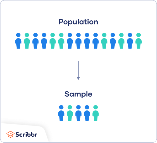
In most cases, it’s too difficult or expensive to collect data from every member of the population you’re interested in studying. Instead, you’ll collect data from a sample.
Statistical analysis allows you to apply your findings beyond your own sample as long as you use appropriate sampling procedures. You should aim for a sample that is representative of the population.
Sampling for statistical analysis
There are two main approaches to selecting a sample.
- Probability sampling: every member of the population has a chance of being selected for the study through random selection.
- Non-probability sampling: some members of the population are more likely than others to be selected for the study because of criteria such as convenience or voluntary self-selection.
In theory, for highly generalizable findings, you should use a probability sampling method. Random selection reduces several types of research bias, like sampling bias, and ensures that data from your sample is actually typical of the population. Parametric tests can be used to make strong statistical inferences when data are collected using probability sampling.
But in practice, it’s rarely possible to gather the ideal sample. While non-probability samples are more likely to at risk for biases like self-selection bias, they are much easier to recruit and collect data from. Non-parametric tests are more appropriate for non-probability samples, but they result in weaker inferences about the population.
If you want to use parametric tests for non-probability samples, you have to make the case that:
- your sample is representative of the population you’re generalizing your findings to.
- your sample lacks systematic bias.
Keep in mind that external validity means that you can only generalize your conclusions to others who share the characteristics of your sample. For instance, results from Western, Educated, Industrialized, Rich and Democratic samples (e.g., college students in the US) aren’t automatically applicable to all non-WEIRD populations.
If you apply parametric tests to data from non-probability samples, be sure to elaborate on the limitations of how far your results can be generalized in your discussion section.
Create an appropriate sampling procedure
Based on the resources available for your research, decide on how you’ll recruit participants.
- Will you have resources to advertise your study widely, including outside of your university setting?
- Will you have the means to recruit a diverse sample that represents a broad population?
- Do you have time to contact and follow up with members of hard-to-reach groups?
Your participants are self-selected by their schools. Although you’re using a non-probability sample, you aim for a diverse and representative sample.
Your participants volunteer for the survey, making this a non-probability sample.
Calculate sufficient sample size
Before recruiting participants, decide on your sample size either by looking at other studies in your field or using statistics. A sample that’s too small may be unrepresentative of the sample, while a sample that’s too large will be more costly than necessary.
There are many sample size calculators online. Different formulas are used depending on whether you have subgroups or how rigorous your study should be (e.g., in clinical research). As a rule of thumb, a minimum of 30 units or more per subgroup is necessary.
To use these calculators, you have to understand and input these key components:
- Significance level (alpha): the risk of rejecting a true null hypothesis that you are willing to take, usually set at 5%.
- Statistical power: the probability of your study detecting an effect of a certain size if there is one, usually 80% or higher.
- Expected effect size: a standardized indication of how large the expected result of your study will be, usually based on other similar studies.
- Population standard deviation: an estimate of the population parameter based on a previous study or a pilot study of your own.
Step 3: Summarize your data with descriptive statistics
Once you’ve collected all of your data, you can inspect them and calculate descriptive statistics that summarize them.
Inspect your data
There are various ways to inspect your data, including the following:
- Organizing data from each variable in frequency distribution tables.
- Displaying data from a key variable in a bar chart to view the distribution of responses.
- Visualizing the relationship between two variables using a scatter plot.
By visualizing your data in tables and graphs, you can assess whether your data follow a skewed or normal distribution and whether there are any outliers or missing data.
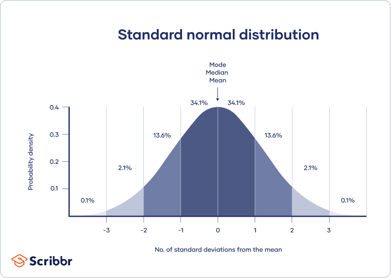
A normal distribution means that your data are symmetrically distributed around a center where most values lie, with the values tapering off at the tail ends.
In contrast, a skewed distribution is asymmetric and has more values on one end than the other. The shape of the distribution is important to keep in mind because only some descriptive statistics should be used with skewed distributions.
Extreme outliers can also produce misleading statistics, so you may need a systematic approach to dealing with these values.
Calculate measures of central tendency
Measures of central tendency describe where most of the values in a data set lie. Three main measures of central tendency are often reported:
- Mode: the most popular response or value in the data set.
- Median: the value in the exact middle of the data set when ordered from low to high.
- Mean: the sum of all values divided by the number of values.
However, depending on the shape of the distribution and level of measurement, only one or two of these measures may be appropriate. For example, many demographic characteristics can only be described using the mode or proportions, while a variable like reaction time may not have a mode at all.
Calculate measures of variability
Measures of variability tell you how spread out the values in a data set are. Four main measures of variability are often reported:
- Range: the highest value minus the lowest value of the data set.
- Interquartile range: the range of the middle half of the data set.
- Standard deviation: the average distance between each value in your data set and the mean.
- Variance: the square of the standard deviation.
Once again, the shape of the distribution and level of measurement should guide your choice of variability statistics. The interquartile range is the best measure for skewed distributions, while standard deviation and variance provide the best information for normal distributions.
Using your table, you should check whether the units of the descriptive statistics are comparable for pretest and posttest scores. For example, are the variance levels similar across the groups? Are there any extreme values? If there are, you may need to identify and remove extreme outliers in your data set or transform your data before performing a statistical test.
| Pretest scores | Posttest scores | |
|---|---|---|
| Mean | 68.44 | 75.25 |
| Standard deviation | 9.43 | 9.88 |
| Variance | 88.96 | 97.96 |
| Range | 36.25 | 45.12 |
| N | 30 | |
From this table, we can see that the mean score increased after the meditation exercise, and the variances of the two scores are comparable. Next, we can perform a statistical test to find out if this improvement in test scores is statistically significant in the population.
It’s important to check whether you have a broad range of data points. If you don’t, your data may be skewed towards some groups more than others (e.g., high academic achievers), and only limited inferences can be made about a relationship.
| Parental income (USD) | GPA | |
|---|---|---|
| Mean | 62,100 | 3.12 |
| Standard deviation | 15,000 | 0.45 |
| Variance | 225,000,000 | 0.16 |
| Range | 8,000–378,000 | 2.64–4.00 |
| N | 653 | |
Next, we can compute a correlation coefficient and perform a statistical test to understand the significance of the relationship between the variables in the population.
Step 4: Test hypotheses or make estimates with inferential statistics
A number that describes a sample is called a statistic, while a number describing a population is called a parameter. Using inferential statistics, you can make conclusions about population parameters based on sample statistics.
Researchers often use two main methods (simultaneously) to make inferences in statistics.
- Estimation: calculating population parameters based on sample statistics.
- Hypothesis testing: a formal process for testing research predictions about the population using samples.
Estimation
You can make two types of estimates of population parameters from sample statistics:
- A point estimate: a value that represents your best guess of the exact parameter.
- An interval estimate: a range of values that represent your best guess of where the parameter lies.
If your aim is to infer and report population characteristics from sample data, it’s best to use both point and interval estimates in your paper.
You can consider a sample statistic a point estimate for the population parameter when you have a representative sample (e.g., in a wide public opinion poll, the proportion of a sample that supports the current government is taken as the population proportion of government supporters).
There’s always error involved in estimation, so you should also provide a confidence interval as an interval estimate to show the variability around a point estimate.
A confidence interval uses the standard error and the z score from the standard normal distribution to convey where you’d generally expect to find the population parameter most of the time.
Hypothesis testing
Using data from a sample, you can test hypotheses about relationships between variables in the population. Hypothesis testing starts with the assumption that the null hypothesis is true in the population, and you use statistical tests to assess whether the null hypothesis can be rejected or not.
Statistical tests determine where your sample data would lie on an expected distribution of sample data if the null hypothesis were true. These tests give two main outputs:
- A test statistic tells you how much your data differs from the null hypothesis of the test.
- A p value tells you the likelihood of obtaining your results if the null hypothesis is actually true in the population.
Statistical tests come in three main varieties:
- Comparison tests assess group differences in outcomes.
- Regression tests assess cause-and-effect relationships between variables.
- Correlation tests assess relationships between variables without assuming causation.
Your choice of statistical test depends on your research questions, research design, sampling method, and data characteristics.
Parametric tests
Parametric tests make powerful inferences about the population based on sample data. But to use them, some assumptions must be met, and only some types of variables can be used. If your data violate these assumptions, you can perform appropriate data transformations or use alternative non-parametric tests instead.
A regression models the extent to which changes in a predictor variable results in changes in outcome variable(s).
- A simple linear regression includes one predictor variable and one outcome variable.
- A multiple linear regression includes two or more predictor variables and one outcome variable.
Comparison tests usually compare the means of groups. These may be the means of different groups within a sample (e.g., a treatment and control group), the means of one sample group taken at different times (e.g., pretest and posttest scores), or a sample mean and a population mean.
- A t test is for exactly 1 or 2 groups when the sample is small (30 or less).
- A z test is for exactly 1 or 2 groups when the sample is large.
- An ANOVA is for 3 or more groups.
The z and t tests have subtypes based on the number and types of samples and the hypotheses:
- If you have only one sample that you want to compare to a population mean, use a one-sample test.
- If you have paired measurements (within-subjects design), use a dependent (paired) samples test.
- If you have completely separate measurements from two unmatched groups (between-subjects design), use an independent (unpaired) samples test.
- If you expect a difference between groups in a specific direction, use a one-tailed test.
- If you don’t have any expectations for the direction of a difference between groups, use a two-tailed test.
The only parametric correlation test is Pearson’s r. The correlation coefficient (r) tells you the strength of a linear relationship between two quantitative variables.
However, to test whether the correlation in the sample is strong enough to be important in the population, you also need to perform a significance test of the correlation coefficient, usually a t test, to obtain a p value. This test uses your sample size to calculate how much the correlation coefficient differs from zero in the population.
You use a dependent-samples, one-tailed t test to assess whether the meditation exercise significantly improved math test scores. The test gives you:
- a t value (test statistic) of 3.00
- a p value of 0.0028
Although Pearson’s r is a test statistic, it doesn’t tell you anything about how significant the correlation is in the population. You also need to test whether this sample correlation coefficient is large enough to demonstrate a correlation in the population.
A t test can also determine how significantly a correlation coefficient differs from zero based on sample size. Since you expect a positive correlation between parental income and GPA, you use a one-sample, one-tailed t test. The t test gives you:
- a t value of 3.08
- a p value of 0.001

Step 5: Interpret your results
The final step of statistical analysis is interpreting your results.
Statistical significance
In hypothesis testing, statistical significance is the main criterion for forming conclusions. You compare your p value to a set significance level (usually 0.05) to decide whether your results are statistically significant or non-significant.
Statistically significant results are considered unlikely to have arisen solely due to chance. There is only a very low chance of such a result occurring if the null hypothesis is true in the population.
This means that you believe the meditation intervention, rather than random factors, directly caused the increase in test scores.
Note that correlation doesn’t always mean causation, because there are often many underlying factors contributing to a complex variable like GPA. Even if one variable is related to another, this may be because of a third variable influencing both of them, or indirect links between the two variables.
A large sample size can also strongly influence the statistical significance of a correlation coefficient by making very small correlation coefficients seem significant.
Effect size
A statistically significant result doesn’t necessarily mean that there are important real life applications or clinical outcomes for a finding.
In contrast, the effect size indicates the practical significance of your results. It’s important to report effect sizes along with your inferential statistics for a complete picture of your results. You should also report interval estimates of effect sizes if you’re writing an APA style paper.
With a Cohen’s d of 0.72, there’s medium to high practical significance to your finding that the meditation exercise improved test scores.
Because your value is between 0.1 and 0.3, your finding of a relationship between parental income and GPA represents a very small effect and has limited practical significance.
Decision errors
Type I and Type II errors are mistakes made in research conclusions. A Type I error means rejecting the null hypothesis when it’s actually true, while a Type II error means failing to reject the null hypothesis when it’s false.
You can aim to minimize the risk of these errors by selecting an optimal significance level and ensuring high power. However, there’s a trade-off between the two errors, so a fine balance is necessary.
Frequentist versus Bayesian statistics
Traditionally, frequentist statistics emphasizes null hypothesis significance testing and always starts with the assumption of a true null hypothesis.
However, Bayesian statistics has grown in popularity as an alternative approach in the last few decades. In this approach, you use previous research to continually update your hypotheses based on your expectations and observations.
Bayes factor compares the relative strength of evidence for the null versus the alternative hypothesis rather than making a conclusion about rejecting the null hypothesis or not.
Other interesting articles
If you want to know more about statistics, methodology, or research bias, make sure to check out some of our other articles with explanations and examples.
Statistics
Methodology