Chi-Square Test of Independence | Formula, Guide & Examples
A chi-square (Χ2) test of independence is a nonparametric hypothesis test. You can use it to test whether two categorical variables are related to each other.
The city decides to test two interventions: an educational flyer (pamphlet) or a phone call. They randomly select 300 households and randomly assign them to the flyer, phone call, or control group (no intervention). They’ll use the results of their experiment to decide which intervention to use for the whole city.
The city plans to use a chi-square test of independence to test whether the proportion of households who recycle differs between the interventions.
Table of contents
- What is the chi-square test of independence?
- Chi-square test of independence hypotheses
- When to use the chi-square test of independence
- How to calculate the test statistic (formula)
- How to perform the chi-square test of independence
- When to use a different test
- Practice questions
- Other interesting articles
- Frequently asked questions about the chi-square test of independence
What is the chi-square test of independence?
A chi-square (Χ2) test of independence is a type of Pearson’s chi-square test. Pearson’s chi-square tests are nonparametric tests for categorical variables. They’re used to determine whether your data are significantly different from what you expected.
You can use a chi-square test of independence, also known as a chi-square test of association, to determine whether two categorical variables are related. If two variables are related, the probability of one variable having a certain value is dependent on the value of the other variable.
The chi-square test of independence calculations are based on the observed frequencies, which are the numbers of observations in each combined group.
The test compares the observed frequencies to the frequencies you would expect if the two variables are unrelated. When the variables are unrelated, the observed and expected frequencies will be similar.
Contingency tables
When you want to perform a chi-square test of independence, the best way to organize your data is a type of frequency distribution table called a contingency table.
A contingency table, also known as a cross tabulation or crosstab, shows the number of observations in each combination of groups. It also usually includes row and column totals.
| Household address | Intervention | Outcome |
|---|---|---|
| 25 Elm Street | Flyer | Recycles |
| 100 Cedar Street | Control | Recycles |
| 3 Maple Street | Control | Does not recycle |
| 123 Oak Street | Phone call | Recycles |
| … | … | … |
They reorganize the data into a contingency table:
| Intervention | Recycles | Does not recycle | Row totals |
|---|---|---|---|
| Flyer (pamphlet) | 89 | 9 | 98 |
| Phone call | 84 | 8 | 92 |
| Control | 86 | 24 | 110 |
| Column totals | 259 | 41 | N = 300 |
They also visualize their data in a bar graph:

Here's why students love Scribbr's proofreading services
Chi-square test of independence hypotheses
The chi-square test of independence is an inferential statistical test, meaning that it allows you to draw conclusions about a population based on a sample. Specifically, it allows you to conclude whether two variables are related in the population.
Like all hypothesis tests, the chi-square test of independence evaluates a null and alternative hypothesis. The hypotheses are two competing answers to the question “Are variable 1 and variable 2 related?”
- Null hypothesis (H0): Variable 1 and variable 2 are not related in the population; The proportions of variable 1 are the same for different values of variable 2.
- Alternative hypothesis (Ha): Variable 1 and variable 2 are related in the population; The proportions of variable 1 are not the same for different values of variable 2.
You can use the above sentences as templates. Replace variable 1 and variable 2 with the names of your variables.
- Null hypothesis (H0): Whether a household recycles and the type of intervention they receive are not related in the population; The proportion of households that recycle is the same for all interventions.
- Alternative hypothesis (Ha): Whether a household recycles and the type of intervention they receive are related in the population; The proportion of households that recycle is not the same for all interventions.
Expected values
A chi-square test of independence works by comparing the observed and the expected frequencies. The expected frequencies are such that the proportions of one variable are the same for all values of the other variable.
You can calculate the expected frequencies using the contingency table. The expected frequency for row r and column c is:

| Intervention | Recycles | Does not recycle | Row totals |
|---|---|---|---|
| Flyer (pamphlet) |  |
 |
 |
 |
 |
||
| Phone call |  |
 |
 |
 |
 |
||
| Control |  |
 |
 |
 |
 |
||
| Column totals |  |
 |
 |
The expected frequencies are such that the proportion of households who recycle is the same for all interventions: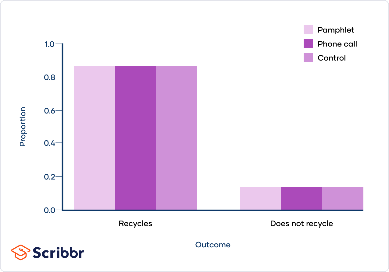
When to use the chi-square test of independence
The following conditions are necessary if you want to perform a chi-square goodness of fit test:
- You want to test a hypothesis about the relationship between two categorical variables (binary, nominal, or ordinal).
- The sample was randomly selected from the population.
- There are a minimum of five observations expected in each combined group.
- They want to test a hypothesis about the relationships between two categorical variables: whether a household recycles and the type of intervention.
- They recruited a random sample of 300 households.
- There are a minimum of five observations expected in each combined group. The smallest expected frequency is 12.57.
How to calculate the test statistic (formula)
Pearson’s chi-square (Χ2) is the test statistic for the chi-square test of independence:

Where
- Χ2 is the chi-square test statistic
- Σ is the summation operator (it means “take the sum of”)
- O is the observed frequency
- E is the expected frequency
The chi-square test statistic measures how much your observed frequencies differ from the frequencies you would expect if the two variables are unrelated. It is large when there’s a big difference between the observed and expected frequencies (O − E in the equation).
Follow these five steps to calculate the test statistic:
Step 1: Create a table
Create a table with the observed and expected frequencies in two columns.
| Intervention | Outcome | Observed | Expected |
|---|---|---|---|
| Flyer | Recycles | 89 | 84.61 |
| Does not recycle | 9 | 13.39 | |
| Phone call | Recycles | 84 | 79.43 |
| Does not recycle | 8 | 12.57 | |
| Control | Recycles | 86 | 94.97 |
| Does not recycle | 24 | 15.03 |
Step 2: Calculate O − E
In a new column called “O − E”, subtract the expected frequencies from the observed frequencies.
| Intervention | Outcome | Observed | Expected | O − E |
|---|---|---|---|---|
| Flyer | Recycles | 89 | 84.61 | 4.39 |
| Does not recycle | 9 | 13.39 | -4.39 | |
| Phone call | Recycles | 84 | 79.43 | 4.57 |
| Does not recycle | 8 | 12.57 | -4.57 | |
| Control | Recycles | 86 | 94.97 | -8.97 |
| Does not recycle | 24 | 15.03 | 8.97 |
Step 3: Calculate (O – E)2
In a new column called “(O − E)2”, square the values in the previous column.
| Intervention | Outcome | Observed | Expected | O − E | (O − E)2 |
|---|---|---|---|---|---|
| Flyer | Recycles | 89 | 84.61 | 4.39 | 19.27 |
| Does not recycle | 9 | 13.39 | -4.39 | 19.27 | |
| Phone call | Recycles | 84 | 79.43 | 4.57 | 20.88 |
| Does not recycle | 8 | 12.57 | -4.57 | 20.88 | |
| Control | Recycles | 86 | 94.97 | -8.97 | 80.46 |
| Does not recycle | 24 | 15.03 | 8.97 | 80.46 |
Step 4: Calculate (O − E)2 / E
In a final column called “(O − E)2 / E”, divide the previous column by the expected frequencies.
| Intervention | Outcome | Observed | Expected | O − E | (O − E)2 | (O − E)2 / E |
|---|---|---|---|---|---|---|
| flyer | Recycles | 89 | 84.61 | 4.39 | 19.27 | 0.23 |
| Does not recycle | 9 | 13.39 | -4.39 | 19.27 | 1.44 | |
| Phone call | Recycles | 84 | 79.43 | 4.57 | 20.88 | 0.26 |
| Does not recycle | 8 | 12.57 | -4.57 | 20.88 | 1.66 | |
| Control | Recycles | 86 | 94.97 | -8.97 | 80.46 | 0.85 |
| Does not recycle | 24 | 15.03 | 8.97 | 80.46 | 5.35 |
Step 5: Calculate Χ2
Finally, add up the values of the previous column to calculate the chi-square test statistic (Χ2).
Χ2 = 9.79

How to perform the chi-square test of independence
If the test statistic is big enough then you should conclude that the observed frequencies are not what you’d expect if the variables are unrelated. But what counts as big enough?
We compare the test statistic to a critical value from a chi-square distribution to decide whether it’s big enough to reject the null hypothesis that the two variables are unrelated. This procedure is called the chi-square test of independence.
Follow these steps to perform a chi-square test of independence (the first two steps have already been completed for the recycling example):
Step 1: Calculate the expected frequencies
Use the contingency table to calculate the expected frequencies following the formula:

Step 2: Calculate chi-square
Use the Pearson’s chi-square formula to calculate the test statistic:

Step 3: Find the critical chi-square value
You can find the critical value in a chi-square critical value table or using statistical software. You need to known two numbers to find the critical value:
- The degrees of freedom (df): For a chi-square test of independence, the df is (number of variable 1 groups − 1) * (number of variable 2 groups − 1).
- Significance level (α): By convention, the significance level is usually .05.
For a test of significance at α = .05 and df = 2, the Χ2 critical value is 5.99.
Step 4: Compare the chi-square value to the critical value
Is the test statistic big enough to reject the null hypothesis? Compare it to the critical value to find out.
Critical value = 5.99
The Χ2 value is greater than the critical value.
Step 5: Decide whether to reject the null hypothesis
- If the Χ2 value is greater than the critical value, then the difference between the observed and expected distributions is statistically significant (p < α).
- The data allows you to reject the null hypothesis that the variables are unrelated and provides support for the alternative hypothesis that the variables are related.
- If the Χ2 value is less than the critical value, then the difference between the observed and expected distributions is not statistically significant (p > α).
- The data doesn’t allow you to reject the null hypothesis that the variables are unrelated and doesn’t provide support for the alternative hypothesis that the variables are related.
There is a significant difference between the observed frequencies and the frequencies expected if the two variables were unrelated (p < .05). This suggests that the proportion of households that recycle is not the same for all interventions.
The city concludes that their interventions have an effect on whether households choose to recycle.
Step 6: Follow up with post hoc tests (optional)
If there are more than two groups in either of the variables and you rejected the null hypothesis, you may want to investigate further with post hoc tests. A post hoc test is a follow-up test that you perform after your initial analysis.
Similar to a one-way ANOVA with more than two groups, a significant difference doesn’t tell you which groups’ proportions are significantly different from each other.
One post hoc approach is to compare each pair of groups using chi-square tests of independence and a Bonferroni correction. A Bonferroni correction is when you divide your original significance level (usually .05) by the number of tests you’re performing.
| Chi-square test of independence | Chi-square test statistic |
|---|---|
| Flyer vs. phone call | 0.014 |
| Flyer vs. control | 6.198 |
| Phone call vs. control | 6.471 |
- Since there are two intervention groups and two outcome groups for each test, there is (2 − 1) * (2 − 1) = 1 degree of freedom.
- There are three tests, so the significance level with a Bonferroni correction applied is α = .05 / 3 = .016.
- For a test of significance at α = .016 and df = 1, the Χ2 critical value is 5.803.
- The chi-square value is greater than the critical value for the pamphlet vs control and phone call vs. control tests.
Based on these findings, the city concludes that a significantly greater proportion of households recycled after receiving a pamphlet or phone call compared to the control.
There was no significant difference in proportion between the pamphlet and phone call intervention, so the city chooses the phone call intervention because it creates less paper waste.
When to use a different test
Several tests are similar to the chi-square test of independence, so it may not always be obvious which to use. The best choice will depend on your variables, your sample size, and your hypotheses.
When to use the chi-square goodness of fit test
There are two types of Pearson’s chi-square test. The chi-square test of independence is one of them, and the chi-square goodness of fit test is the other. The math is the same for both tests—the main difference is how you calculate the expected values.
You should use the chi-square goodness of fit test when you have one categorical variable and you want to test a hypothesis about its distribution.
When to use Fisher’s exact test
If you have a small sample size (N < 100), Fisher’s exact test is a better choice. You should especially opt for Fisher’s exact test when your data doesn’t meet the condition of a minimum of five observations expected in each combined group.
When to use McNemar’s test
You should use McNemar’s test when you have a closely-related pair of categorical variables that each have two groups. It allows you to test whether the proportions of the variables are equal. This test is most often used to compare before and after observations of the same individuals.
When to use a G test
A G test and a chi-square test give approximately the same results. G tests can accommodate more complex experimental designs than chi-square tests. However, the tests are usually interchangeable and the choice is mostly a matter of personal preference.
One reason to prefer chi-square tests is that they’re more familiar to researchers in most fields.
Practice questions
Do you want to test your knowledge about the chi-square goodness of fit test? Download our practice questions and examples with the buttons below.
Download Word doc Download Google doc
Other interesting articles
If you want to know more about statistics, methodology, or research bias, make sure to check out some of our other articles with explanations and examples.
Statistics
Methodology
Frequently asked questions about the chi-square test of independence
Cite this Scribbr article
If you want to cite this source, you can copy and paste the citation or click the “Cite this Scribbr article” button to automatically add the citation to our free Citation Generator.
Turney, S. (2023, June 22). Chi-Square Test of Independence | Formula, Guide & Examples. Scribbr. Retrieved July 23, 2026, from https://www.scribbr.com/statistics/chi-square-test-of-independence/