How to Find Degrees of Freedom | Definition & Formula
Degrees of freedom, often represented by v or df, is the number of independent pieces of information used to calculate a statistic. It’s calculated as the sample size minus the number of restrictions.
Degrees of freedom are normally reported in brackets beside the test statistic, alongside the results of the statistical test.
The test statistic, t, has 9 degrees of freedom:
df = n − 1
df = 10 − 1
df = 9
You calculate a t value of 1.41 for the sample, which corresponds to a p value of .19. You report your results:
“The participants’ mean daily calcium intake did not differ from the recommended amount of 1000 mg, t(9) = 1.41, p = 0.19.”
What are degrees of freedom?
In inferential statistics, you estimate a parameter of a population by calculating a statistic of a sample. The number of independent pieces of information used to calculate the statistic is called the degrees of freedom. The degrees of freedom of a statistic depend on the sample size:
- When the sample size is small, there are only a few independent pieces of information, and therefore only a few degrees of freedom.
- When the sample size is large, there are many independent pieces of information, and therefore many degrees of freedom.
When you estimate a parameter, you need to introduce restrictions in how values are related to each other. As a result, the pieces of information are not all independent. To put it another way, the values in the sample are not all free to vary.
The following analogy and example show you what it means for a value to be free to vary and how it’s affected by restrictions.
Free to vary: Dessert analogy
By deciding to have a different dessert every day, your roommate is imposing a restriction on her dessert choices.
On Monday, she can choose any of the seven desserts. On Tuesday, she can choose any of the six remaining dessert options. On Wednesday, she can choose any of the five remaining options, and so on.
By Sunday, she’s had all the dessert options except one. She doesn’t have any choice to make on Sunday since there’s only one option remaining.
Due to her restriction, your roommate could only choose her dessert on six of the seven days. Her dessert choice was free to vary on these six day. In contrast, her dessert choice on the last day wasn’t free to vary; it depended on her dessert choices of the previous six days.
Free to vary: Sum example
The requirement of summing to 100 is a restriction on your number choices.
For the first number, you can choose any integer you want. Whatever your choice, the sum of the five numbers can still be 100. This is also true of the second, third, and fourth numbers.
You have no choice for the final number; it has only one possible value and it isn’t free to vary. For example, imagine you chose 15, 27, 42, and 3 as your first four numbers. For the numbers to sum to 100, the final number needs to be 13.
Due to the restriction, you could only choose four of the five numbers. The first four numbers were free to vary. In contrast, the fifth number wasn’t free to vary; it depended on the other four numbers.
Here's why students love Scribbr's proofreading services
Degrees of freedom and hypothesis testing
The degrees of freedom of a test statistic determines the critical value of the hypothesis test. The critical value is calculated from the null distribution and is a cut-off value to decide whether to reject the null hypothesis.
The degrees of freedom affect the critical value by changing the shape of the null distribution. The null distributions of Student’s t, chi-square, and other test statistics change with the degrees of freedom, but they each change in different ways.
Student’s t distribution
To perform a t test, you calculate t for the sample and compare it to a critical value. To find the right critical value, you need to use the Student’s t distribution with the appropriate degrees of freedom.
The null distribution of Student’s t changes with the degrees of freedom:
- When df = 1, the distribution is strongly leptokurtic, meaning the probability of extreme values is greater than in a normal distribution.
- As the df increases, the distribution becomes narrower and less leptokurtic. It becomes increasing similar to a standard normal distribution
- When df ≥ 30, Student’s t distribution is almost the same as a standard normal distribution. If you have a sample size of greater than 30, you can use the standard normal distribution (also known as the z distribution) instead of Student’s t distribution.
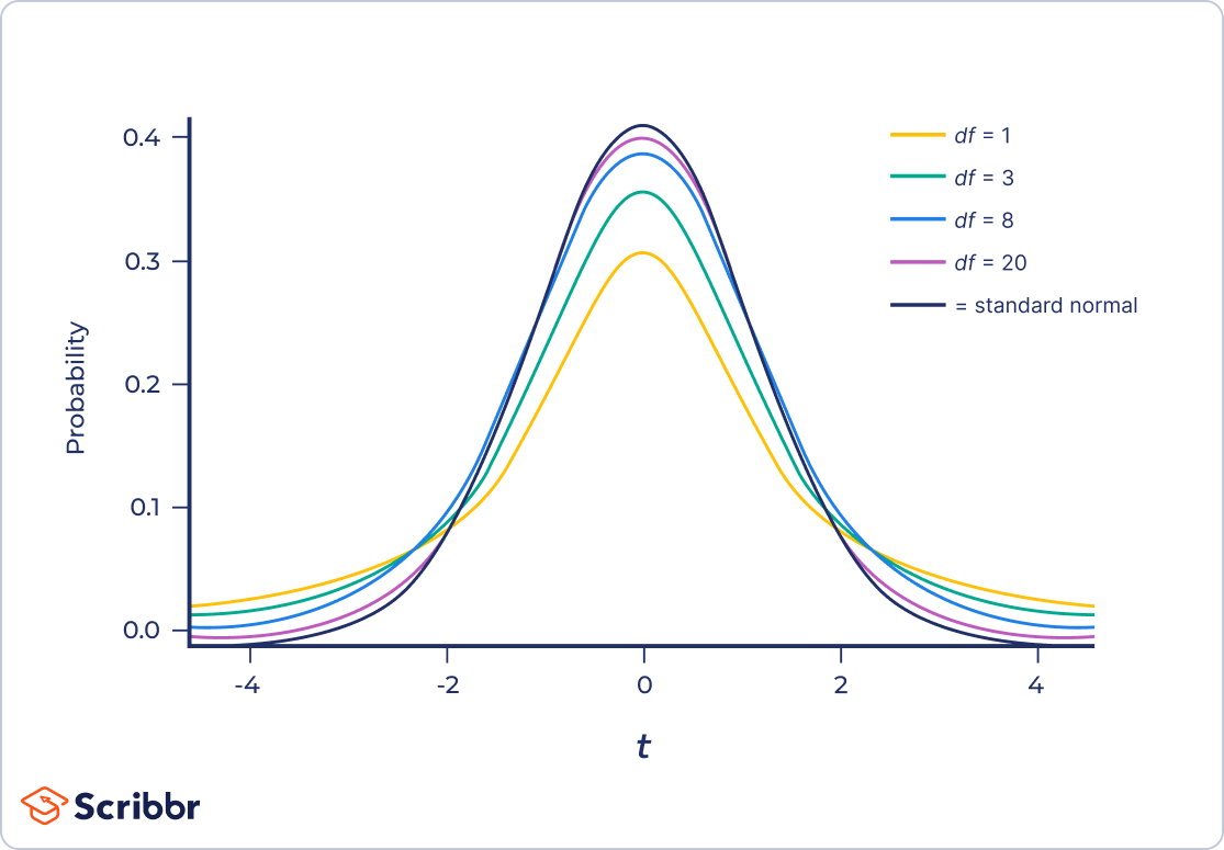
This change in the distribution’s shape makes intuitive sense. The t distribution has less spread as the number of degrees of freedom increases because the certainty of the estimate increases. Imagine repeatedly sampling the population and calculating Student’s t; the larger the sample size, the less the test statistic will vary between samples.
You take a random sample of 10 adults and measure their daily calcium intake.
The one-sample t test determines when a population mean is different from a certain value. However, you don’t know the population mean, so first you need to estimate it using the sample mean. You calculate that the sample mean is 820 mg.
By assuming the population mean has a certain value, you impose a restriction on the sample: the values in the sample must have a mean of 820 mg. Consequently, the final value isn’t free to vary; it only has one possible value.
For example, imagine the nine of the ten people in the sample have daily calcium intakes of 410, 1230, 870, 1110, 570, 390, 1030, 1080, and 630 mg. The tenth person must have a daily calcium intake of 880 mg for the sample to have a mean of 820 mg.
Because of the restriction, only nine values in the sample are free to vary. The test statistic, t, has nine degrees of freedom.
To find the critical value, you need to use the t distribution for nine degrees of freedom. If the sample’s t is greater than the critical value, then you reject the null hypothesis.
Chi-square distribution
To perform a chi-square test, you compare a sample’s chi-square to a critical value. To find the right critical value, you need to use the chi-square distribution with the appropriate degrees of freedom.
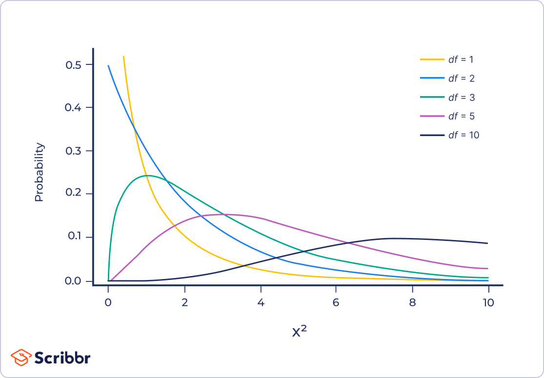
The null distribution of chi-square changes with the degrees of freedom, but in a different way than Student’s t distribution:
- When df < 3, the probability distribution is shaped like a backwards “J.”
- When df ≥ 3, the probability distribution is hump-shaped, with the peak of the hump located at Χ2 = df − 2. The hump is right-skewed, meaning that the distribution is longer on the right side of its peak.
- When df > 90, the chi-square distribution is approximated by a normal distribution.
How to calculate degrees of freedom
The degrees of freedom of a statistic is the sample size minus the number of restrictions. Most of the time, the restrictions are parameters that are estimated as intermediate steps in calculating the statistic.
n − r
Where:
- n is the sample size
- r is the number of restrictions, usually the same as the number of parameters estimated
The degrees of freedom can’t be negative. As a result, the number of parameters you estimate can’t be larger than your sample size.
Test-specific formulas
It can be difficult to figure out the number of restrictions. It’s often easier to use test-specific formulas to figure out the degrees of freedom of a test statistic.
The table below gives formulas to calculate the degrees of freedom for several commonly-used tests.
| Test | Formula | Notes |
|---|---|---|
| One-sample t test | df = n − 1 | |
| Independent samples t test | df = n1 + n2 − 2 | Where n1 is the sample size of group 1 and n2 is the sample size of group 2 |
| Dependent samples t test | df = n − 1 | Where n is the number of pairs |
| Simple linear regression | df = n − 2 | |
| Chi-square goodness of fit test | df = k − 1 | Where k is the number of groups |
| Chi-square test of independence | df = (r − 1) * (c − 1) | Where r is the number of rows (groups of one variable) and c is the number of columns (groups of the other variable) in the contingency table |
| One-way ANOVA | Between-group df = k − 1 Within-group df = N − k Total df = N − 1 |
Where k is the number of groups and N is the sum of all groups’ sample sizes |
Degrees of freedom quiz
Here's why students love Scribbr's proofreading services
Other interesting articles
If you want to know more about statistics, methodology, or research bias, make sure to check out some of our other articles with explanations and examples.
Statistics
Methodology
Frequently asked questions about degrees of freedom
Cite this Scribbr article
If you want to cite this source, you can copy and paste the citation or click the “Cite this Scribbr article” button to automatically add the citation to our free Citation Generator.
Turney, S. (2023, June 22). How to Find Degrees of Freedom | Definition & Formula. Scribbr. Retrieved July 1, 2026, from https://www.scribbr.com/statistics/degrees-of-freedom/