Pearson Correlation Coefficient (r) | Guide & Examples
The Pearson correlation coefficient (r) is the most common way of measuring a linear correlation. It is a number between –1 and 1 that measures the strength and direction of the relationship between two variables.
| Pearson correlation coefficient (r) | Correlation type | Interpretation | Example |
|---|---|---|---|
| Between 0 and 1 | Positive correlation | When one variable changes, the other variable changes in the same direction. | Baby length & weight:
The longer the baby, the heavier their weight. |
| 0 | No correlation | There is no relationship between the variables. | Car price & width of windshield wipers:
The price of a car is not related to the width of its windshield wipers. |
| Between 0 and –1 |
Negative correlation | When one variable changes, the other variable changes in the opposite direction. | Elevation & air pressure:
The higher the elevation, the lower the air pressure. |
Table of contents
- What is the Pearson correlation coefficient?
- Visualizing the Pearson correlation coefficient
- When to use the Pearson correlation coefficient
- Calculating the Pearson correlation coefficient
- Testing for the significance of the Pearson correlation coefficient
- Reporting the Pearson correlation coefficient
- Other interesting articles
- Frequently asked questions about the Pearson correlation coefficient
What is the Pearson correlation coefficient?
The Pearson correlation coefficient (r) is the most widely used correlation coefficient and is known by many names:
- Pearson’s r
- Bivariate correlation
- Pearson product-moment correlation coefficient (PPMCC)
- The correlation coefficient
The Pearson correlation coefficient is a descriptive statistic, meaning that it summarizes the characteristics of a dataset. Specifically, it describes the strength and direction of the linear relationship between two quantitative variables.
Although interpretations of the relationship strength (also known as effect size) vary between disciplines, the table below gives general rules of thumb:
| Pearson correlation coefficient (r) value | Strength | Direction |
|---|---|---|
| Greater than .5 | Strong | Positive |
| Between .3 and .5 | Moderate | Positive |
| Between 0 and .3 | Weak | Positive |
| 0 | None | None |
| Between 0 and –.3 | Weak | Negative |
| Between –.3 and –.5 | Moderate | Negative |
| Less than –.5 | Strong | Negative |
The Pearson correlation coefficient is also an inferential statistic, meaning that it can be used to test statistical hypotheses. Specifically, we can test whether there is a significant relationship between two variables.
Here's why students love Scribbr's proofreading services
Visualizing the Pearson correlation coefficient
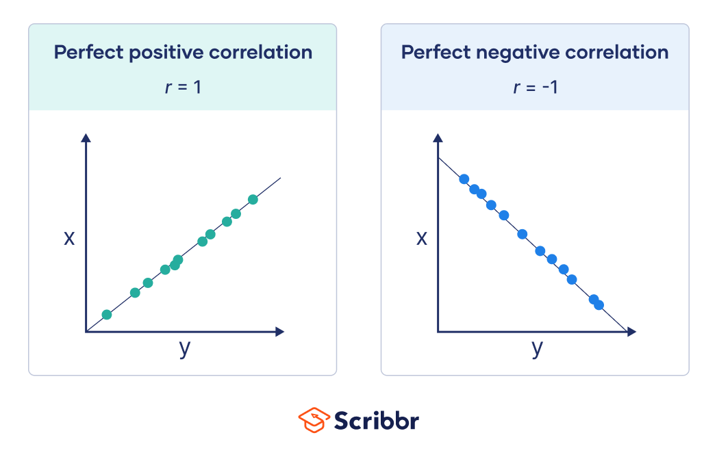
Another way to think of the Pearson correlation coefficient (r) is as a measure of how close the observations are to a line of best fit.
The Pearson correlation coefficient also tells you whether the slope of the line of best fit is negative or positive. When the slope is negative, r is negative. When the slope is positive, r is positive.
When r is 1 or –1, all the points fall exactly on the line of best fit:
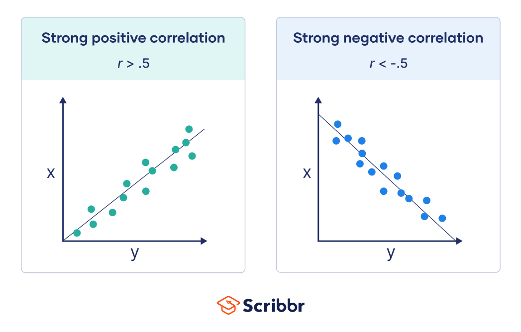
When r is greater than .5 or less than –.5, the points are close to the line of best fit:
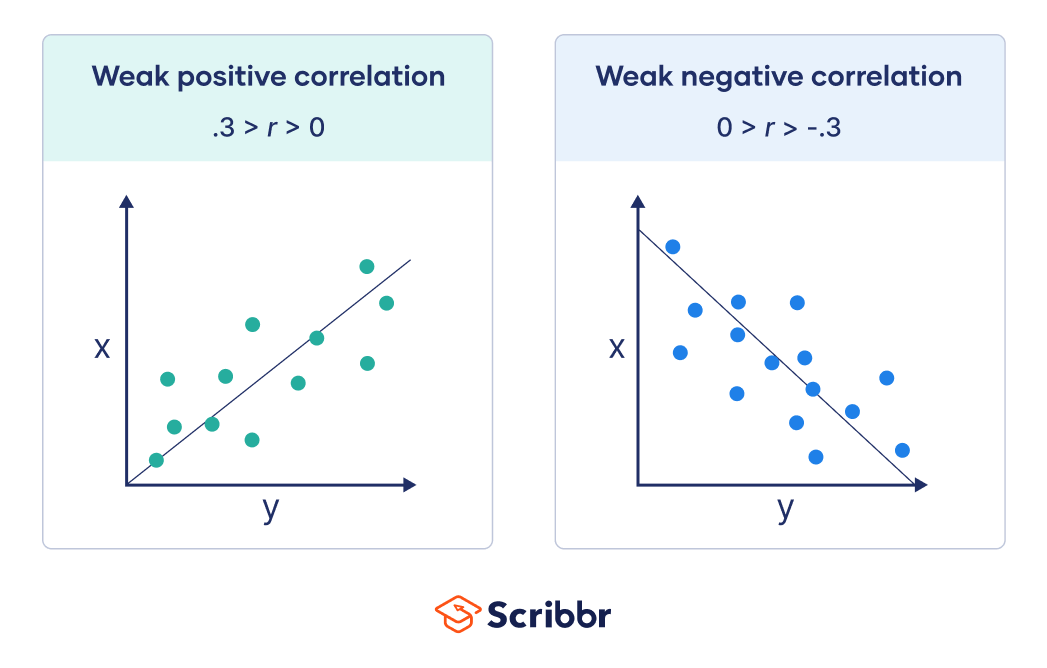
When r is between 0 and .3 or between 0 and –.3, the points are far from the line of best fit:
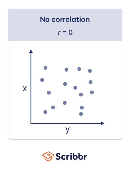
When r is 0, a line of best fit is not helpful in describing the relationship between the variables:
When to use the Pearson correlation coefficient
The Pearson correlation coefficient (r) is one of several correlation coefficients that you need to choose between when you want to measure a correlation. The Pearson correlation coefficient is a good choice when all of the following are true:
- Both variables are quantitative: You will need to use a different method if either of the variables is qualitative.
- The variables are normally distributed: You can create a histogram of each variable to verify whether the distributions are approximately normal. It’s not a problem if the variables are a little non-normal.
- The data have no outliers: Outliers are observations that don’t follow the same patterns as the rest of the data. A scatterplot is one way to check for outliers—look for points that are far away from the others.
- The relationship is linear: “Linear” means that the relationship between the two variables can be described reasonably well by a straight line. You can use a scatterplot to check whether the relationship between two variables is linear.
Pearson vs. Spearman’s rank correlation coefficients
Spearman’s rank correlation coefficient is another widely used correlation coefficient. It’s a better choice than the Pearson correlation coefficient when one or more of the following is true:
- The variables are ordinal.
- The variables aren’t normally distributed.
- The data includes outliers.
- The relationship between the variables is non-linear and monotonic.
Calculating the Pearson correlation coefficient
Below is a formula for calculating the Pearson correlation coefficient (r):
![\begin{equation*} r = \frac{ n\sum{xy}-(\sum{x})(\sum{y})}{% \sqrt{[n\sum{x^2}-(\sum{x})^2][n\sum{y^2}-(\sum{y})^2]}} \end{equation*}](https://www.scribbr.com/wp-content/ql-cache/quicklatex.com-a916dc6277f04e962bf89d6e60f745ec_l3.png "Rendered by QuickLaTeX.com")
The formula is easy to use when you follow the step-by-step guide below. You can also use software such as R or Excel to calculate the Pearson correlation coefficient for you.
| Weight (kg) | Length (cm) |
|---|---|
| 3.63 | 53.1 |
| 3.02 | 49.7 |
| 3.82 | 48.4 |
| 3.42 | 54.2 |
| 3.59 | 54.9 |
| 2.87 | 43.7 |
| 3.03 | 47.2 |
| 3.46 | 45.2 |
| 3.36 | 54.4 |
| 3.3 | 50.4 |
Step 1: Calculate the sums of x and y
Start by renaming the variables to “x” and “y.” It doesn’t matter which variable is called x and which is called y—the formula will give the same answer either way.
Next, add up the values of x and y. (In the formula, this step is indicated by the Σ symbol, which means “take the sum of”.)
Length = y
Σx = 3.63 + 3.02 + 3.82 + 3.42 + 3.59 + 2.87 + 3.03 + 3.46 + 3.36 + 3.30
Σx = 33.5
Σy = 53.1 + 49.7 + 48.4 + 54.2 + 54.9 + 43.7 + 47.2 + 45.2 + 54.4 + 50.4
Σy = 501.2
Step 2: Calculate x2 and y2 and their sums
Create two new columns that contain the squares of x and y. Take the sums of the new columns.
| x | y | x2 | y2 |
|---|---|---|---|
| 3.63 | 53.1 | (3.63)2 = 13.18 | (53.1)2 = 2 819.6 |
| 3.02 | 49.7 | 9.12 | 2 470.1 |
| 3.82 | 48.4 | 14.59 | 2 342.6 |
| 3.42 | 54.2 | 11.7 | 2 937.6 |
| 3.59 | 54.9 | 12.89 | 3 014 |
| 2.87 | 43.7 | 8.24 | 1 909.7 |
| 3.03 | 47.2 | 9.18 | 2 227.8 |
| 3.46 | 45.2 | 11.97 | 2 043 |
| 3.36 | 54.4 | 11.29 | 2 959.4 |
| 3.3 | 50.4 | 10.89 | 2 540.2 |
Σx2 = 13.18 + 9.12 + 14.59 + 11.70 + 12.89 + 8.24 + 9.18 + 11.97 + 11.29 + 10.89
Σx2 = 113.05
Σy2 = 2 819.6 + 2 470.1 + 2 342.6 + 2 937.6 + 3 014.0 + 1 909.7 + 2 227.8 + 2 043.0 + 2 959.4 + 2 540.2
Σy2 = 25 264
Step 3: Calculate the cross product and its sum
In a final column, multiply together x and y (this is called the cross product). Take the sum of the new column.
| x | y | x2 | y2 | xy (x*y) |
|---|---|---|---|---|
| 3.63 | 53.1 | 13.18 | 2 819.6 | 3.63 * 53.1 = 192.8 |
| 3.02 | 49.7 | 9.12 | 2 470.1 | 150.1 |
| 3.82 | 48.4 | 14.59 | 2 342.6 | 184.9 |
| 3.42 | 54.2 | 11.7 | 2 937.6 | 185.4 |
| 3.59 | 54.9 | 12.89 | 3 014 | 197.1 |
| 2.87 | 43.7 | 8.24 | 1 909.7 | 125.4 |
| 3.03 | 47.2 | 9.18 | 2 227.8 | 143 |
| 3.46 | 45.2 | 11.97 | 2 043 | 156.4 |
| 3.36 | 54.4 | 11.29 | 2 959.4 | 182.8 |
| 3.3 | 50.4 | 10.89 | 2 540.2 | 166.3 |
Σxy = 192.8 + 150.1 + 184.9 + 185.4 + 197.1 + 125.4 + 143.0 + 156.4 + 182.8 + 166.3
Σxy = 1 684.2
Step 4: Calculate r
Use the formula and the numbers you calculated in the previous steps to find r.


![r = \frac{ n\sum{xy}-(\sum{x})(\sum{y})}{% \sqrt{[n\sum{x^2}-(\sum{x})^2][n\sum{y^2}-(\sum{y})^2]}}](https://www.scribbr.com/wp-content/ql-cache/quicklatex.com-ab89c0ce832838d8e949743001780a76_l3.png "Rendered by QuickLaTeX.com")
![r = \frac{ 10\sum{1\,684.2}-(33.5)(501.2)}{% \sqrt{[(10)(113.05)-(33.5)^2][(10)(25\,264)-(501.2)^2]}}](https://www.scribbr.com/wp-content/ql-cache/quicklatex.com-afe81c87b865bc391c72805b2a147642_l3.png "Rendered by QuickLaTeX.com")
![r = \frac{ 16\,842-16\,790.2)}{% \sqrt{[1\,130.5-1\,122.25][252\,640-251\,201.4]}}](https://www.scribbr.com/wp-content/ql-cache/quicklatex.com-a93d69120752d4a79c1cd3bc22266aff_l3.png "Rendered by QuickLaTeX.com")


Testing for the significance of the Pearson correlation coefficient
The Pearson correlation coefficient can also be used to test whether the relationship between two variables is significant.
The Pearson correlation of the sample is r. It is an estimate of rho (ρ), the Pearson correlation of the population. Knowing r and n (the sample size), we can infer whether ρ is significantly different from 0.
- Null hypothesis (H0): ρ = 0
- Alternative hypothesis (Ha): ρ ≠ 0
To test the hypotheses, you can either use software like R or Stata or you can follow the three steps below.
Step 1: Calculate the t value
Calculate the t value (a test statistic) using this formula:


Step 2: Find the critical value of t
You can find the critical value of t (t*) in a t table. To use the table, you need to know three things:
- The degrees of freedom (df): For Pearson correlation tests, the formula is df = n – 2.
- Significance level (α): By convention, the significance level is usually .05.
- One-tailed or two-tailed: Most often, two-tailed is an appropriate choice for correlations.
Step 3: Compare the t value to the critical value
Determine if the absolute t value is greater than the critical value of t. “Absolute” means that if the t value is negative you should ignore the minus sign.
t* = 2.306
The t value is less than the critical value of t.
Step 4: Decide whether to reject the null hypothesis
- If the t value is greater than the critical value, then the relationship is statistically significant (p < α). The data allows you to reject the null hypothesis and provides support for the alternative hypothesis.
- If the t value is less than the critical value, then the relationship is not statistically significant (p > α). The data doesn’t allow you to reject the null hypothesis and doesn’t provide support for the alternative hypothesis.
(Note that a sample size of 10 is very small. It’s possible that you would find a significant relationship if you increased the sample size.)
Reporting the Pearson correlation coefficient
If you decide to include a Pearson correlation (r) in your paper or thesis, you should report it in your results section. You can follow these rules if you want to report statistics in APA Style:
- You don’t need to provide a reference or formula since the Pearson correlation coefficient is a commonly used statistic.
- You should italicize r when reporting its value.
- You shouldn’t include a leading zero (a zero before the decimal point) since the Pearson correlation coefficient can’t be greater than one or less than negative one.
- You should provide two significant digits after the decimal point.
When Pearson’s correlation coefficient is used as an inferential statistic (to test whether the relationship is significant), r is reported alongside its degrees of freedom and p value. The degrees of freedom are reported in parentheses beside r.
Other interesting articles
If you want to know more about statistics, methodology, or research bias, make sure to check out some of our other articles with explanations and examples.
Statistics
Methodology
Frequently asked questions about the Pearson correlation coefficient
Cite this Scribbr article
If you want to cite this source, you can copy and paste the citation or click the “Cite this Scribbr article” button to automatically add the citation to our free Citation Generator.
Turney, S. (2024, February 10). Pearson Correlation Coefficient (r) | Guide & Examples. Scribbr. Retrieved June 16, 2026, from https://www.scribbr.com/statistics/pearson-correlation-coefficient/